When to stop and when to keep going
I was recently posed the following puzzle:
Imagine you are offered a choice between two different bets. In (A), you must make 2/3 soccer shots, and in (B), you must make 5/8. In either case, you receive a \($100\) prize for winning the bet. Which bet should you choose?
Intuitively, a professional soccer player would want to take the second bet, whereas a hopeless case like me would want to take the first. However, suppose you have no idea whether your skill level is closer to Lionel Messi or to Max Shinn. The puzzle continues:
You are offered the option to take practice shots to determine your skill level at a cost of \($0.01\) for each shot. Assuming you and the goalie never fatigue, how do you decide when to stop taking practice shots and choose a bet?
Clearly it is never advisable to take more than \(100/.01=10000\) practice shots, but how many should we take? A key to this question is that you do not have to determine the number of shots to take beforehand. Therefore, rather than determining a fixed number of shots to take, we will instead need to determine a decision procedure for when to stop shooting and choose a bet.
There is no single “correct” answer to this puzzle, so I have documented my approach below.
Approach
To understand my approach, first realize that there are a finite number of potential states that the game can be in, and that you can fully define each state based on how many shots you have made and how many you have missed. The sum of these is the total number of shots you have taken, and the order does not matter. Additionally, we assume that all states exist, even if you will never arrive at that state by the decision procedure.
An example of a state is taking 31 shots, making 9 of them, and missing 22 of them. Another example is taking 98 shots, making 1 of them and missing 97 of them. Even though we may have already made a decision before taking 98 shots, the concept of a state does not depend on the procedure used to “get there”.
Using this framework, it is sufficient to show which decision we should take given what state we are in. My approach is as follows:
- Find a tight upper bound \(B \ll 10000\) on the number of practice shots to take. This limits the number of states to work with.
- Determine the optimal choice based on each potential state after taking \(B\) total shots. Once \(B\) shots have been taken, it is always best to have chosen either bet (A) or bet (B), so choose the best bet without the option of shooting again.
- Working backwards, starting with states with \(B-1\) shots and moving down to \(B-2,...,0\), determine the expected value of each of the three choices: select bet (A), select bet (B), or shoot again. Use this to determine the optimal choice to make at that position.
The advantage of this approach is that the primary criterion we will work with is the expected value for each decision. This means that if we play the game many times we will maximize the amount of money we earn. As a convenient consequence of this, we know much money we can expect to earn given our current state.
The only reason this procedure is necessary is because we don’t know our skill level. If we could determine with 100% accuracy what are skill level was, we would never need to take any shots at all. Thus, a key part of this procedure is estimating our skill level.
What if you know your skill level?
We define skill level as the probability \(p_0\) that you will make a shot. So if you knew your probability of making each shot, we could find your expected payoff from each bet. On the plot below, we show the payoff (in dollars) of each bet on the y-axis, and how it changes with skill on the x-axis.
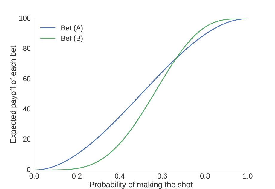
Assuming we have a precise knowledge of your skill level, we can find how much money you can expect to make from each bet.
The first thing to notice is the obvious: as our skill improves, the amount of money we can expect to win increases. Second, we see that there is some point (the “equivalence point”) at which the bets are equal; we compute this numerically to be \(p_0 = 0.6658\). We should choose bet (A) if our skill level is worse than \(0.6658\), and bet (B) if it is greater than \(0.6658\).
But suppose our guess is poor. We notice that the consequence for guessing too high is less than the consequence for guessing too low. It is better to bias your choice towards (A) unless you obtain substantial evidence that you have a high skill level and (B) would be a better choice. In other words, the potential gains from choosing (A) over (B) are larger than the potential gains for choosing (B) over (A).
Finding a tight upper bound
Quantifying this intuition, we compute the maximal possible gain of choosing (A) over (B) and (B) over (A) as the maximum distance between the curves on each side of the equivalence point. In other words, we find the skill level at which the incentive is strongest to choose one bet over the other, and then find what the incentive is at these points.
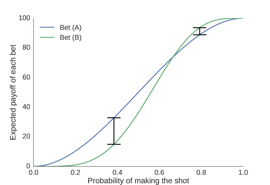
We see here the locations where the distance between the curves is greatest, showing the skill levels where it is most advantageous to choose (A) or (B).
This turns out to be \($4.79\) for choosing (B) over (A), and \($17.92\) for choosing (A) over (B). Since each shot costs \($0.01\), we conclude that it is never a good idea to take more than 479 practice shots. Thus, our upper bound \(B=479\).
Determining the optimal choice at the upper bound
Because we will never take more than 479 shots, we use this as a cutoff point, and force a decision once 479 shots have been taken. So for each possible combinations of successes and failures, we must find whether bet (A) or bet (B) is better.
In order to determine this, we need two pieces of information: first, we need the expected value of bets (A) and (B) given \(p_0\) (i.e. the curve shown above); second, we need the distribution representing our best estimate of \(p_0\). Remember, it is not enough to simply choose (A) when our predicted skill is less than \(0.6658\) and (B) when it is greater than \(0.6658\); since we are biased towards choosing (A), we need a probability distribution representing potential values of \(p_0\). Then, we can find the expected value of each bet given the distribution of \(p_0\) (see appendix for more details). This can be computed with a simple integral, and is easy to approximate numerically.
Once we have performed these computations, in addition to having information about whether (A) or (B) was chosen, we also know the expected value of the chosen bet. This will be critical for determining whether it is beneficial to take more shots before we have reached the upper bound.
Determining the optimal choice below the upper bound
We then go down one level: if 478 shots have been taken, with \(k\) successes and \((478-k)\) failures, should we choose (A), should we choose (B), or should we take another shot? Remember, we would like to select the choice which will give us the highest expected outcome.
Based on this principle, it is only advisable to take another shot if it would influence the outcome; in other words, if you would choose the same bet no matter what the outcome of your next shot, it does not make sense to take another shot, because you lose \($0.01\) without gaining any information. It only makes sense to take the shot if the information gained from taking the shot increases the expected value by more than \($0.01\).
Thus, we would only like to take another shot if the information gained is worth more than \($0.01\). We can compute this by finding the expected value of each of the three options (choose (A), choose (B), or shoot again). Using our previous experiments to judge the probability of a successful shot (see appendix), we can find the expected payoff of taking another shot. If it is greater than choosing (A) or (B), we take the shot.
Working backwards, we continue until we are on our first shot, where we assume we have a \(50\)% chance of succeeding. Once we reach this point, we have a full decision tree, indicating which action we should take based on the outcome of each shot, and the entire decision process can be considered solved.
Conclusion
Here is the decision tree, plotted in raster form.
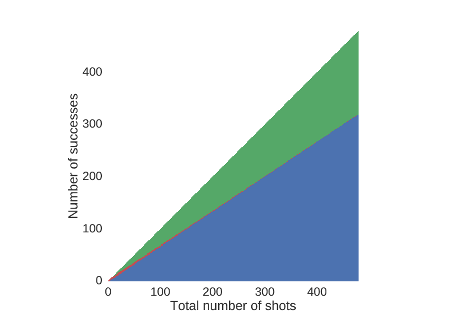
Starting at the point (0,0), go one to the right for every shot that you take, and one up for every shot that you make. Red indicates you should shoot again, blue indicates you should choose (A), and green indicates you should choose (B).
Looking more closely at the beginning, we see that unless you are really good, you should choose (A) rather quickly.
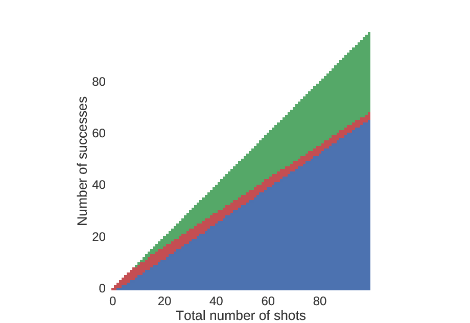
An identical plot to that above, but zoomed in near the beginning.
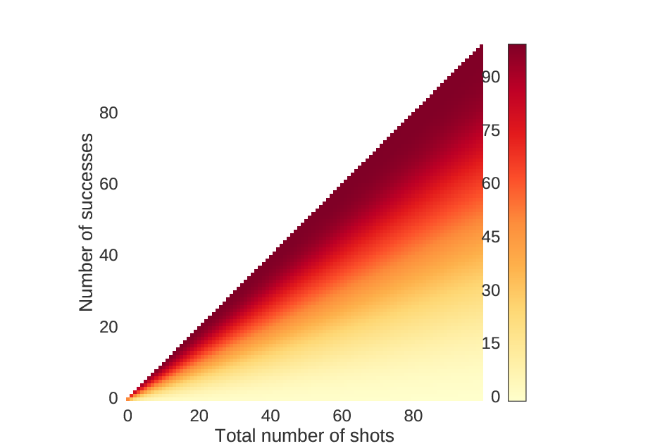
We can also look at the amount of money you will win on average if you play by this strategy. As expected, when you make more shots, you will have a higher chance of winning more money.

For each point in the previous figures, these values correspond to the choices.
We can also look at the zoomed in version.
An identical plot to the one above, but zoomed in near the beginning.
This algorithm grows in memory and computation time like \(O(B^2)\), meaning that if we double the size of the upper bound, we quadruple the amount of memory and CPU time we require.
This may not be the best strategy, but it seems to be a principled strategy which works reasonably well with a relatively small runtime.
Appendix: Determining the distribution of \(p_0\)
In order to find the distribution for \(p_0\), we consider the distribution of \(p_0\) for a single shot. The chance that we make a shot is \(100\)% if \(p_0=1\), \(0\)% if \(p_0=0\), \(50\)% if \(p_0=0.5\), and so on. Thus, the distribution of \(p_0\) from a single successful trial is \(f(p)=p\) for \(0 ≤ p ≤ 1\). Similarly, if we miss the shot, then the distribution is \(f(p)=(1-p)\) for \(0≤p≤1\). Since these probabilities are independent, we can multiply them together and find that, for \(n\) shots, \(k\) successes, and \((n-k)\) failures, we have \(f(p)=p^k (1-p)^{n-k}/c\) for some normalizing constant \(c\). It turns out, this is identical to the beta distribution, with parameters \(α=k+1\) and \(β=n-k+1\).
However, we need a point estimate of \(p_0\) to compute the expected value of taking another shot. We cannot simply use the ratio \(n/k\) for two practical reasons: first, it is undefined when no shots have been taken, and second, when the first shot has been taken, we have a \(100\)% probability of one outcome and a \(0\)% probability of the other. If we want to assume a \(50\)% probability of making the shot initially, an easy way to solve this problem is to use the ratio \((k+1)/(n+2)\) instead of \(k/n\) to estimate the probability. Interestingly, this quick and dirty solution is equivalent to finding the mean of the beta distribution. When no shots have been taken, \(k=0\) and \(n=0\), so \(α=1\) and \(β=1\), which is equivalent to the uniform distribution, hence our non-informative prior.