Which word is the bird?
What do you call a turkey in Turkey? An india! So what do you call an india in India? A peru! English isn’t the only language that likes to name its birds after countries.
Before you ask what you call a peru in Peru, just look at the chart:
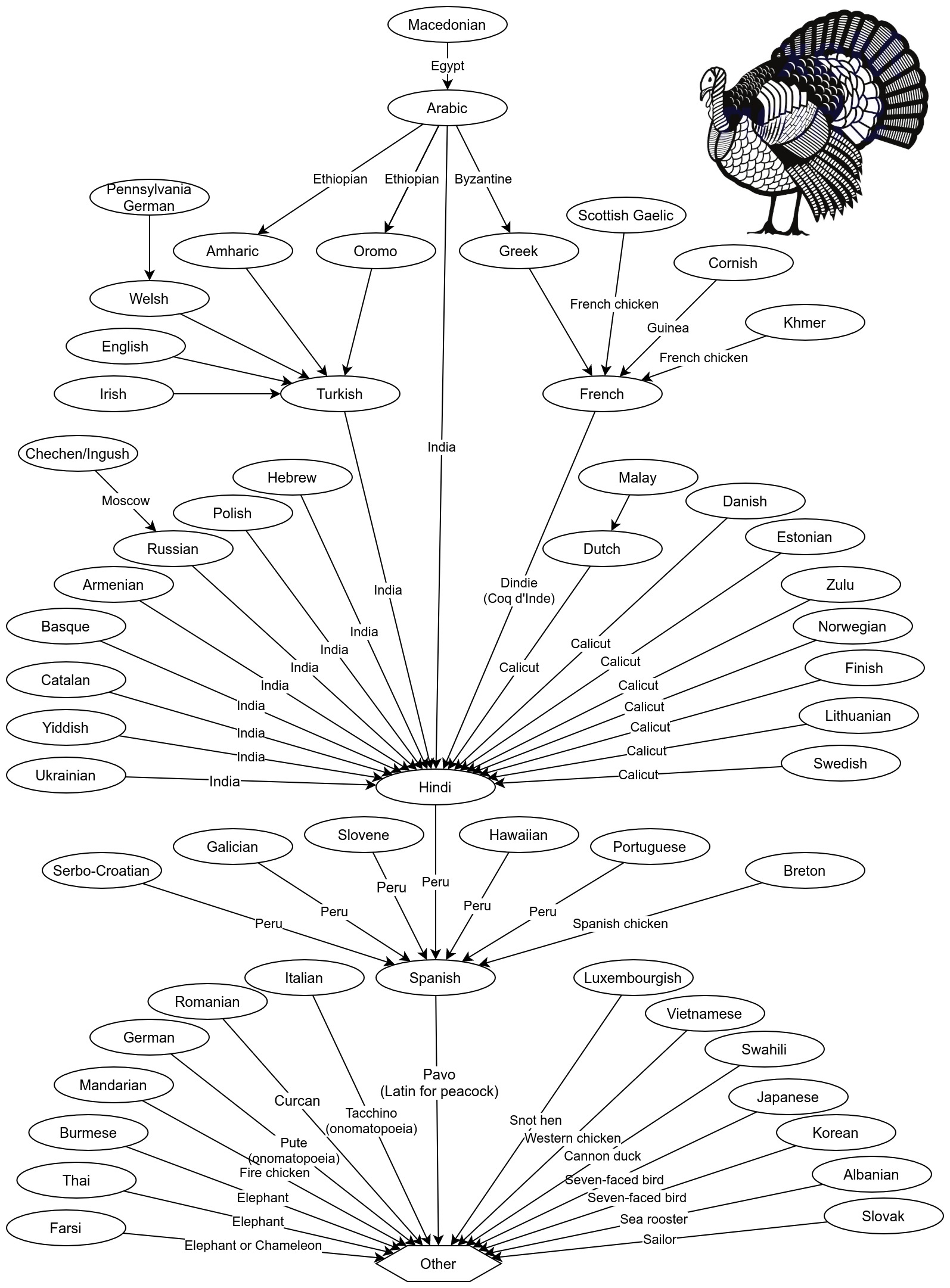
The name for turkey in many different languages.
It turns out most languages name this bird after a foreign country. And when you trace the names from country to country, you almost always end up in Peru.
Is that right?
Well… no, the diagram above is not quite correct. The most important links in the diagram are over-simplified. In particular:
Turkish was not the only widespread language in Turkey when turkeys came to Europe. Three languages were widespread in Turkey at the time: Turkish, Mesopotamian Arabic, and Kurmanji Kurdish. Turkish has two words for “turkey”: one refers to India, and the other is culuk, from an Ottoman word for “woodcock”. Mesopotamian Arabic and Kurmanji Kurdish both have onomatopoeia names: alu alu and elok, respectively. So while some people from Turkey would eventually call a turkey an “india”, not everybody would.
India has many languages. If we exclude Malayalam (see below), many of the most widespread Indian languages call the turkey a “peru”. However, some of them also call it a turkey. And some do not refer to a place at all.
The dominant language in Calicut (now Kozhikode) is Malayalam, not Hindi. Many of the references to India are actually references to the city of Kozhikode (formerly known as Calicut) where Malayalam is the dominant language. Malayalam has different words for turkey than most Indian languages. Three words are in common use: vaan kozhi (literally “mouth chicken”), thurki kozhi (literally “Turkey chicken”) or kalkkam, which comes from the Dutch word, meaning “Calicut”. So, in Kozhikode, they don’t actually call the bird a peru. They call it a mouth chicken, a turkey, or… a kozhikode.
Historically, “India” could have also meant the West Indies. The languages of the pre-Columbian West Indies primarily derived from the Arawakan language family. The most widely spoken of these languages was Taíno. Since it continued to be spoken for many years after colonization, we know the word for turkey was guanaho. (Modern Cuban Spanish still uses the word guanajo, based on the Taíno word.) The proto-Arawakan root for the word “turkey” is thought to be *mara-dii, which would have been either modified or replaced in the various Arawakan languages.
Spanish has many words for turkey. Today, the dominant language in Peru is Spanish, but Spanish has many different words for turkey. The Castilian Spanish word pavo comes from the Latin for peacock, but other names include chompipe, chumpe, gallina de la tierra, gánso, guanajo, guajolote, kókono, picho, pisco, and pípila.
Historically, “Peru” referred to the regions of South America colonized by the Spanish. The area called “Peru” roughly coincided with the Inca Empire, but did not include Mexico, which fell within New Spain. Turkeys were domesticated throughout the Americas long before the arrival of the Spanish. Therefore, instead of Spanish, we need to look at the languages of pre-colonial Peru. While most of these languages are now extinct, two such languages are still spoken today: Quechua and Aymara. The Quechua word for turkey is qallqatu, but it is unclear if this is a modern loan word referring to Kozhikode. The Aymara word for turkey is pawu, and again, it is unknown whether this word existed in pre-Columbian times, whether it derived from the modern Spanish word pavo, or whether it refers to “Peru”, another self-reference. Since turkeys are not native to Peru, the name for turkey may not have even been standardised in these regions.
So, using all of this information, we can construct a more accurate chart.
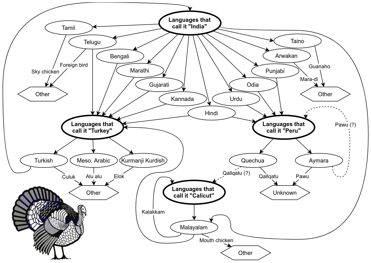
The more accurate name for turkey in many different languages.
This time, the flow through languages can go in loops and circles, and there is no single country at the end.
So where are turkeys actually from?
Turkeys are not native to Peru. In fact, they are not native to any of the lands they are named after. Turkeys are native to North and Central America. By 700 AD, wild turkeys (Meleagris gallopavo gallopavo) were domesticated in Southern Mexico, and by 1500, this domesticated breed of turkey was widespread throughout Mexico, Central America, and parts of northern South America. This is the domesticated breed that the Spanish brought back to Europe in 1511.
Turkeys grew to be very popular in Europe and were widespread by the 1550s. They were so popular that the English colonists brought turkeys with them to New England in the early 1600s. These domesticated turkeys interbred with the much larger wild turkeys in eastern North America (Meleagris gallopavo silvestris). The hybrid turkey, now known as the American Bronze, was then exported from the Americas back to Europe, and from Europe around the world. The hybrid turkeys became even more popular than the original domesticated Mexican turkeys, and are the same turkeys we enjoy today.
Appendix: Turkey naming trivia
In Farsi, one word for turkey is bughalamun, the same as the word for “chameleon”. This word used to be the name of a colourful fabric (a damask). Like chameleons, male turkeys can change the colour of the skin on their head to red, blue, or white. This is due to the arrangement of collagen and blood vessels in their skin.
In Farsi, another word for turkey translates to “elephant bird”, a translation shared with Burmese and Thai. Male turkeys have a “snood”, a long, narrow, dangly flap of skin which hangs over the top of their beak. If you squint, this might resemble an elephant’s trunk. This snood can also contract to form a small horn, resembling a unicorn. All of these colours and shapes on its face earned it the name “seven faced bird” in Japanese and Korean.
In Greek, the translation is literally “French bird”, but the origin of the term “French” is unrelated to France. The Greek name for turkey is galopoula. The suffix poula is a feminine suffix (and pouli can also mean bird), but galo originates from romance languages, meaning cockerel. It is probably a shortened loan word from old romance languages, galo d’India. But in Greek, galo can also mean “French”. So, the Greek the reference to France is just a coincidence, and may truly be a reference to India.
Likewise, in Pennsylvania German, reference to Wales is a coincidence. The literal translation of Welschhinkel is “foreign chicken”, not “Welsh chicken”. In Pennsylvania German, Welsch does not mean Wales, it simply means “foreign”. By coincidence, the word for “foreign” bears an uncanny resemblance to the name of a country, even though the etymologies are different.
Finally, the best false etymology of all: in Malayalam, Kozhikode translates to “chicken castle” (from kozhi and kota)!
Appendix: Words for turkey
The following is a list of different translations of the word “turkey”. I have left out any words which are named after India, Kozhikode, Turkey, and Peru. Some of the languages below may have a second word named after one of these four places, which do not appear in the table, even if those names are more popular than the listed names.
I have confirmed each of these words through multiple sources. When a source is not obvious, I have linked to it.
Places with no native turkeys
| Language | English translation | Word (latin script) | Word (original script) |
|---|---|---|---|
| Albanian | Sea rooster | Gjel Deti | |
| Arabic (Egyptian) | Greek (Byzantine) rooster | Dik rumi | ديك رومي |
| Arabic (Levantine) | Ethiopian (Abyssinian) rooster | Dik al-habas | دِيك الْحَبَش |
| Arabic (Mesopotamian) | (Onomatopoeia) | Alou alou | علوعلو |
| Arabic (Moroccan) | Baby | Bibi | بيبي |
| Breton | Spanish chicken | Yar-Spagn1 | |
| Burmese | Elephant fowl | Krakhcang | ကြက်ဆင် |
| Chechen | Moscow | Moscal | москал |
| Chinese | Fire chicken | Huǒjī (Mandarin), Fo gai (Cantonese) | 火雞 |
| Cornish | Guinea chicken | Yar Gyni | |
| Czech | Rooster (from Proto-Slavic) | Krocan | |
| Farsi | Chameleon, colourful fabric | Buqalamun | بوقلمون |
| Farsi | Elephant bird | Fill Murgh | فیلمرغ |
| German | (Onomatopoeia) | Pute | |
| German | Rooster that says “trut” | Truthahn | |
| Greek | “French” bird | Galopoula | γαλοπούλα |
| Ingush | Moscow | Moscal | москал |
| Italian | (Onomatopoeia) | Tacchino | |
| Japanese | Seven-faced bird | Shichimenchō | 七面鳥 |
| Khmer | French (European) chicken | Mŏən baarang | មាន់បារាំង |
| Korean | Seven-faced bird | Chilmyeonjo | 칠면조 |
| Kurdish (Kurmanji) | (Onomatopoeia) | Elok 2 | |
| Luxembourgish | Snot hen | Schnuddelhong | |
| Macedonian | Egypt | Misir | мисир |
| Malay | Dutch chicken | Ayam belanda | |
| Pennsylvania German | Foreign (Welsh) chicken | Welschhinkel | |
| Quechua | Qallqatu | ||
| Romanian | Rooster (from Proto-Slavic) | Curcan | |
| Scots | (Onomatopoeia) | Bubbly-jock | |
| Scottish Gaelic | French rooster | Coileach-Frangach | |
| Scottish Gaelic | Warrior | Pulaidh | |
| Serbian | Rooster (from Proto-Slavic) | Ćurka | |
| Slovak | Sea/sailor | Moriak | |
| Spanish (Colombia) | Bird (from Quechua) | Pisco | |
| Spanish (Cuba) | (From Taino) | Guanajo | |
| Spanish (El Salvador) | Chumpe | ||
| Spanish (Guatemala) | Chompipe | ||
| Spanish (Mexico) | Picho | ||
| Spanish (Mexico) | Pípila | ||
| Spanish (Mexico) | (From Nahuatl) | Guajolote | |
| Spanish (Mexico, historic) | Local chicken | Gallina de la tierra | |
| Spanish (New Mexico) | (From Nahuatl “turkey chick”) | Kókono | |
| Spanish (New Mexico) | Goose | Gánso | |
| Spanish (Spain) | Peacock (from Latin) | Pavo | |
| Swahili | Cannon duck | Bata mzinga | |
| Tamil | Sky chicken | Van koli | வான்கோழி |
| Taíno | Guanaho | ||
| Telugu | Foreign/border chicken | Seemakodi | సీమకోడి |
| Turkish | (from the word for woodcock) | Culuk | |
| Vietnamese | Foreign (French) chicken | Gà tây |
Places with native turkeys
| Language | English translation | Word (latin script) | Word (original script) |
|---|---|---|---|
| Abenaki | Nahama | ||
| Aymara | Pawu | ||
| Blackfoot | Big bird | Ómahksipi’kssíí | |
| Catawba | Big chicken | Watkątru | |
| Cherokee | Gvna | ᎬᎾ | |
| Chickasaw | (Onomatopoeia) | Chaloklowaꞌ | |
| Choctaw | fakit | ||
| Choctaw | Tall chicken | Aka̱k chaha | |
| Dakota | (Suffix “taŋka” means “big”) | Waglekṡuŋtaŋka | |
| Dakota | (Suffix “taŋka” means “big”) | żicataŋka | |
| Mayan (Classic) | Ak’ach | (See here or here, figure 3) | |
| Mayan (Q’eqchi) | Ak’ach | ||
| Mayan (Kʼicheʼ) | no’s | ||
| Mayan (Yucatec) | Tzo’ | ||
| Mayan (Yucatec) | Ulum | ||
| Mayan (Yucatec) | (Ocellated turkey) | Kutz3 | (See here or here) |
| Miami | Pileewa | ||
| Mohawk | Skaweró:wane | ||
| Mohegan-Pequot | Náham | ||
| Munsee | Pŭléew | ||
| Nahuatl | Huexolotl | ||
| Nahuatl | Totollin | ||
| Navajo | (from “to peck”) | Tązhii | |
| Ojibwe | Big bird | Gichi-bine | |
| Ojibwe | Big bird | Mizise | |
| Shawnee | Pelewa | ||
| Shoshoni | (from “to pick with teeth”) | Guyungiyaa | |
| Unami | Chikënëm |
Sources
History of turkey domestication and etymology: Crawford (1992), Schorger (1966)
Names for Turkey in Spanish: Kiddle (1951) (South America), du Bois (1979) (New Mexico)
Sources for names were numerous and mostly included reputable online dictionaries. Where possible, I cross-checked this real usage based on internet forum posts including: 1 2 3 4
I did not take much information from modern secondary source summaries because I found them to be less accurate, but here are some of them anyway: 1 2 3 4 5 6
Bonus! Some cartoons: Polandball, Itchy Feet
If you find any mistakes or possible additions, please let me know and I will update the article!
Footnotes
-
In Breton, the bird’s name is widely cited to be yar-Spagn (“Spanish chicken”), but this word appears to be rare. The much more common name is yar-Indez (“Indian chicken”). ↩
-
Kurmanji Kurdish Wikipedia claims a few more country names, including Misri (Egyptian, çûkê Misirê) and Shami (Demascus/Syria, çûkê Şamê), but I cannot seem to verify these names. ↩
-
I have included the Yucatec Mayan word “kutz”, even though this word refers specifically to the ocellated turkey, a different (but closely related) species found only on the Yucatan peninsula. ↩
Beyond the overtone series: the overtone grid
The overtone series, also known as the harmonic series, is one of the most fundamental explanations for what makes music sound pleasant. Whenever you hear a note played on a musical instrument, the note isn’t just made of one frequency. The tone you perceive is the base frequency (the “fundamental”). However, the note also consists of overtones, several higher pitched frequencies, which give each musical instrument its distinct sound (its “timbre”). The overtones series is the reason why thick, tightly-voiced chords sound muddy on low-pitched instruments; why the trombone needs to move its slide to play different notes; and why the V7 chord desperately wants to resolve to a I chord.
This post describes how I turned the overtone series into a grid and composed a piece of music based on it. If you just want to hear the piece, you can download the score and listen to a performance by pianist Chiara Naldi.
Reminder: the overtone series
To construct the overtone series, some fundamental frequency \(f_0\) is multiplied by whole numbers. So, the first frequency is \(1 \times f_0\), the second is \(2 \times f_0\), the third is \(3 \times f_0\), and so on:
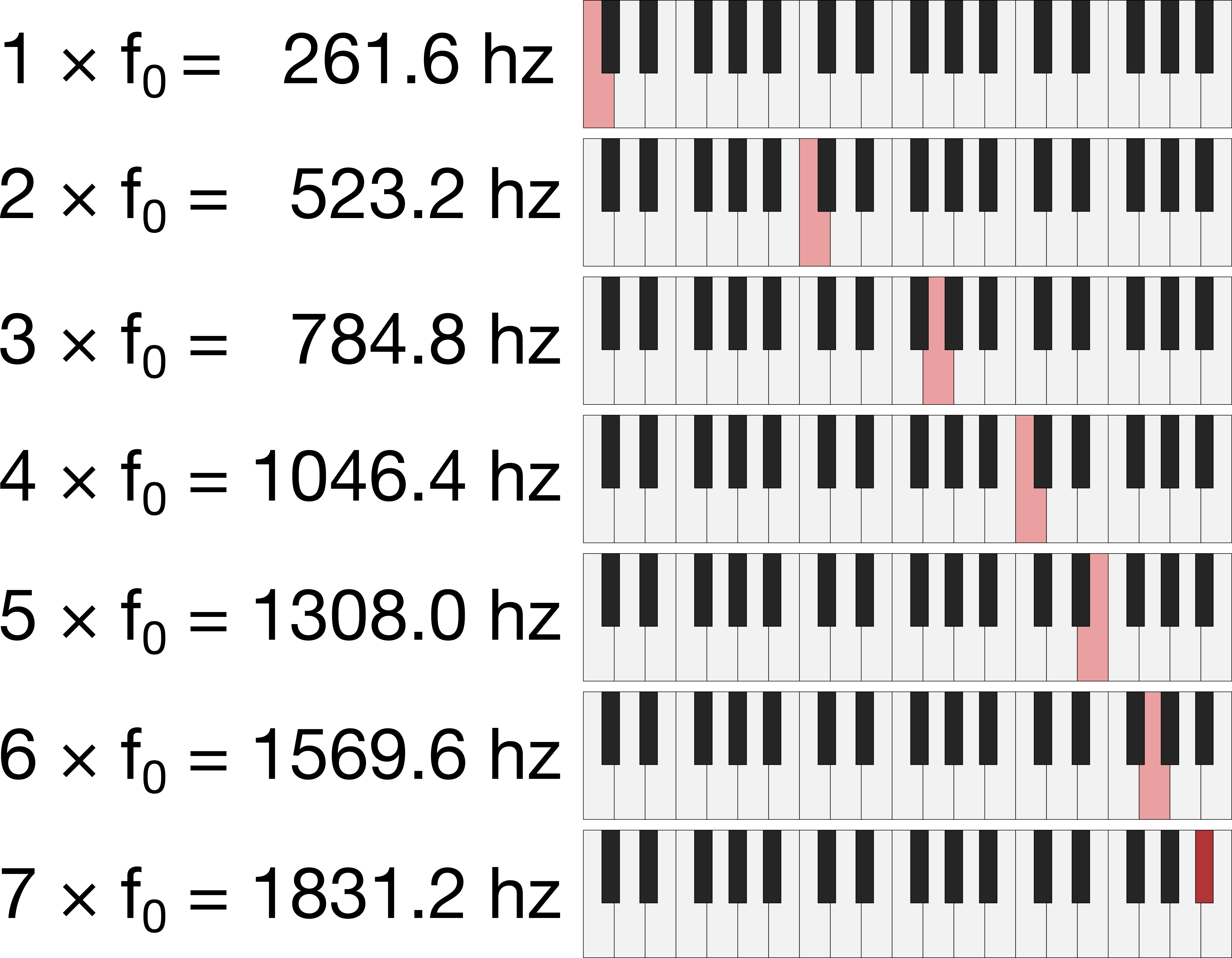
Image of piano keys highlighting the overtone series
Another way to think about the overtone series is as the vibration of a string. Suppose we find a string of length \(L_0\) that vibrates at our fundamental frequency \(f_0\). Then, we cut the string into equal parts, so that each of the new short strings has the same length. If we cut the string in half, each string has length \(L_0/2\), and if we cut it in thirds, the lengths are \(L_0/3\), and so on. More generally, if we cut it into \(N\) equal parts, then each part has a length of:
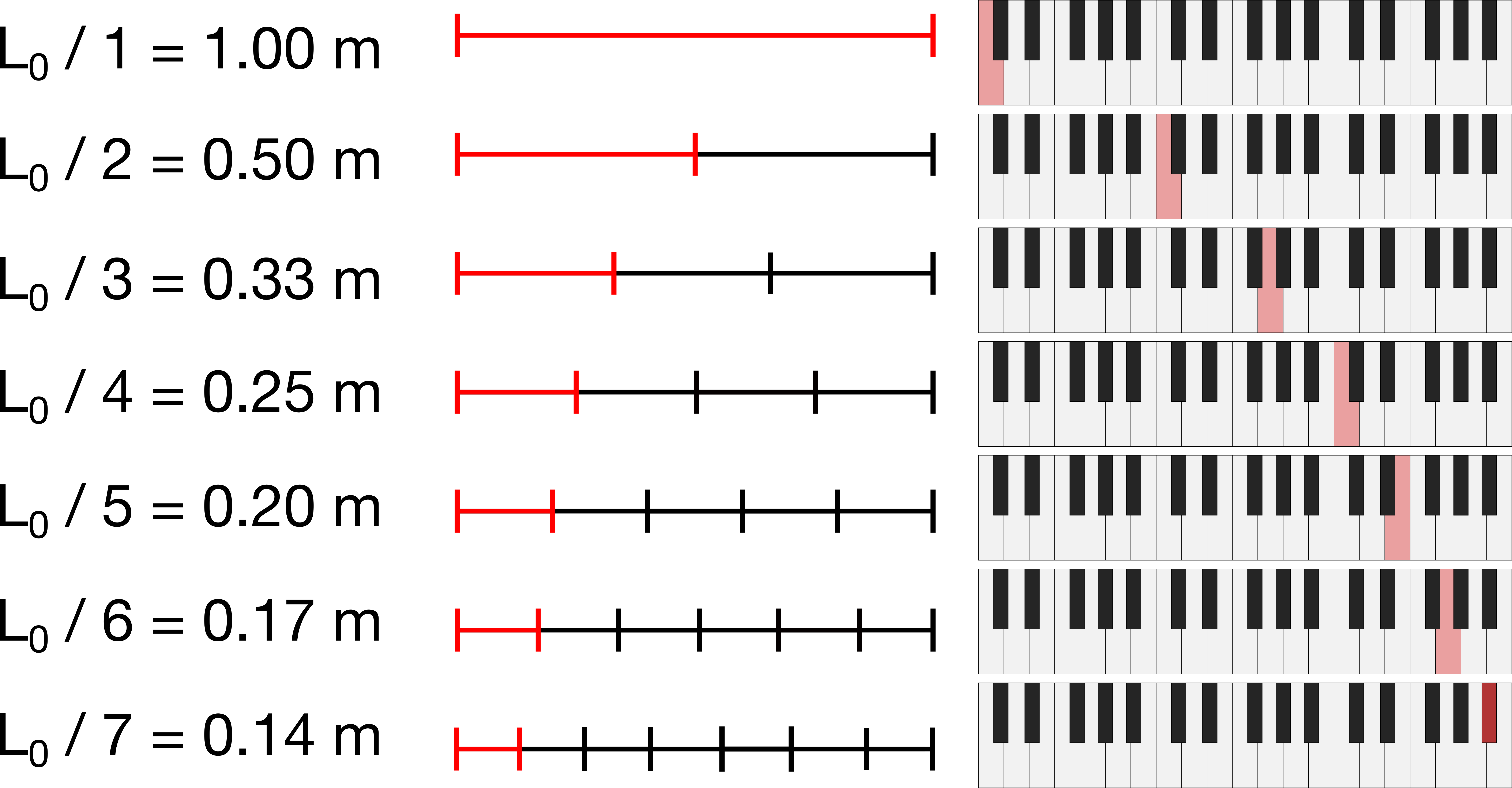
Image of cuts of a violin string highlighting the overtone series
It turns out that a string cut into two equal parts will vibrate at the frequency \(2f_0\), three equal parts will vibrate at \(3f_0\), and \(N\) equal parts will vibrate at \(N f_0\). So, we have two equivalent ways to think about the going up the overtone series: as an even multiple of a fundamental frequency, or as a string being cut. In both of these cases, we have some number (such as 2, 3, or \(N\) in the examples above) which represents the term of the overtone series. We call these the 2nd, 3rd, or \(N\)‘th harmonics.
Generalising the overtone series
In the example above, we divided the string into \(N\) different segments, but we cut each segment to be the same size. What if, instead, we took more than one segment at a time? Now, instead of cutting at every single location where we marked, we look at all of the string lengths which could be made by performing some, but not all, of those cuts. Let’s see what notes could come out of this type of a scheme.
Image of different cuts of a violin string highlighting a generalised overtone series
So, the first two terms do not change: they are still \(L_0\) and \(L_0/2\), corresponding to frequencies \(f_0\) and \(2f_0\). However, the next term will be a bit different. In the standard overtone series, we would have \(L_0/3\), corresponding to a frequency of \(3f_0\). Here, we have two options: the same \(L_0/3\) term with a frequency of \(3f_0\), and a new term, \(2L_0/3\), corresponding to the frequency of \(1.5f_0\). If we go up one more level to \(N=4\), we get a new term as well. We have the familiar \(L_0/4\) term with frequency \(4f\) from the overtone series, and also \(2L_0/4=L_0/2\), a frequency of \(2f\). But we have another new term as well: \(3L_0/4\), with frequency \(1.33f_0\). These frequencies line up approximately with the keys of a piano:
Image of piano keys highlighting a generalised overtone series
We notice that there are two relevant numbers now: the number of pieces we divide the string into (\(N\)), and the number of those pieces we take, which we will call \(M\). According to this scheme, instead of cutting into \(1/N\) segments, we cut into segments of length \(M/N\), where \(M<N\). (This gives us a fraction, a rational number).
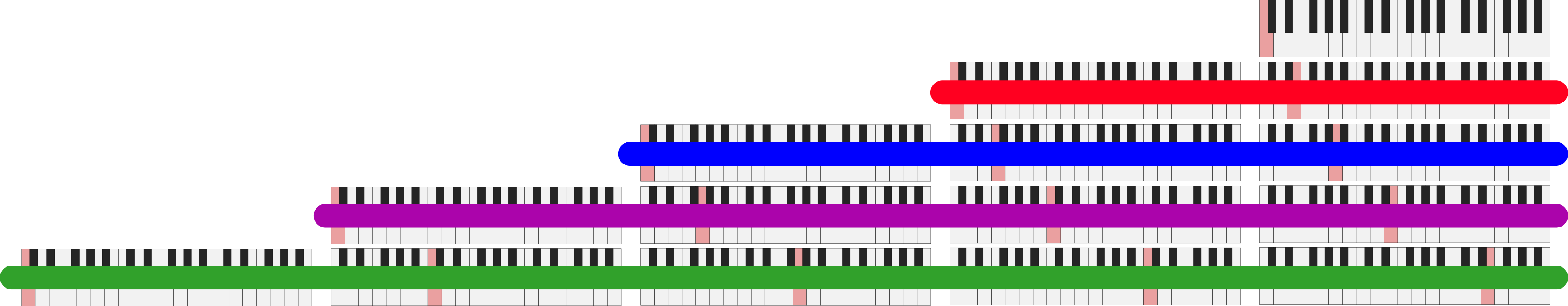
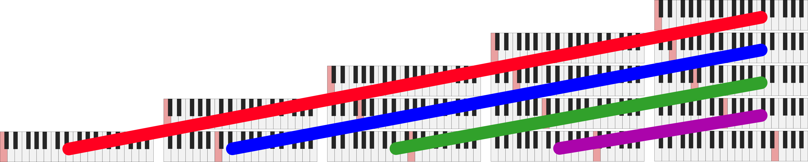
Since we have two numbers instead of one, it is a bit awkward to write them in a list. Instead, we can organise these pitches on a grid. Each column of the grid is \(N\), the number of segments we divide the string into, and each row is a value of \(M\), the number of consecutive segments we take before we cut.
Grid of piano keys showing the overtone grid
Because this generalisation can be arranged on a grid, we obtain not only one series of pitches, but several. We can read the grid up and down, side to side, or diagonally to get lots of different series of notes. This grid forms the basis for Music of the Leaves.
Music of the Leaves
“Music of the Leaves” incorporate each row, column, and diagonal pattern from this grid into a piece of music. It does this by layering them in one note at a time. The piece starts with the first term of the series, the fundamental, and gradually layers in the different notes. When all of the notes have been added, the patterns described above emerge.
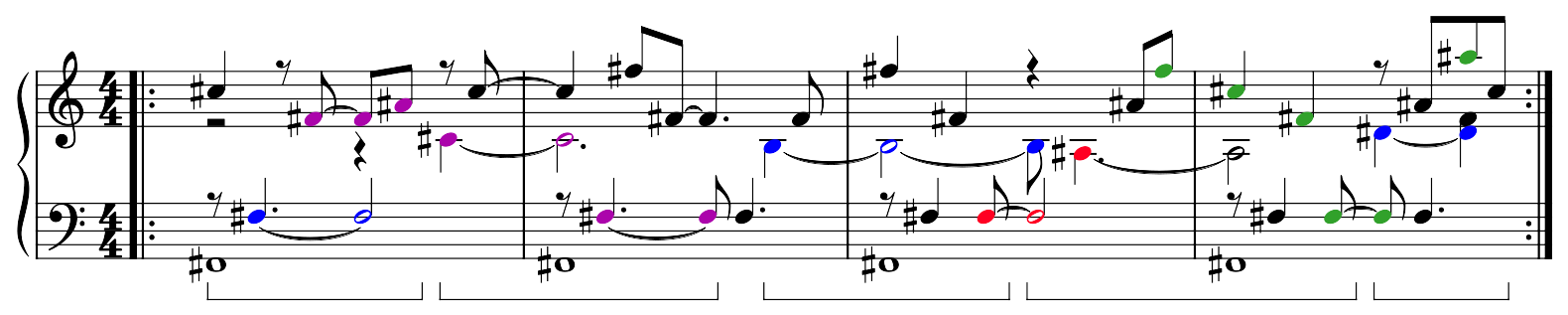
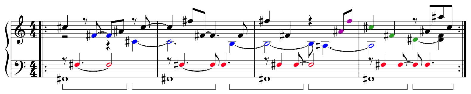
The piece is built exclusively on a repeated four-measure fragment:
Repeated four-measure passage in Music of the Leaves
The four-measure fragment is made from patterns coming from a traversal of the grid in each direction. For instance, consider the four columns:
Traversing the overtone grid by columns
These are represented as patterns in this four-measure segment here:
Notes corresponding to the columns of the overtone grid
We can do the same thing for the rows:
Traversing the overtone grid by rows
These are represented as patterns here:
Notes corresponding to the rows of the overtone grid
And finally for the diagonals:
Traversing the overtone grid by diagonals
We see the patterns here:
Notes corresponding to the diagonals of the overtone grid
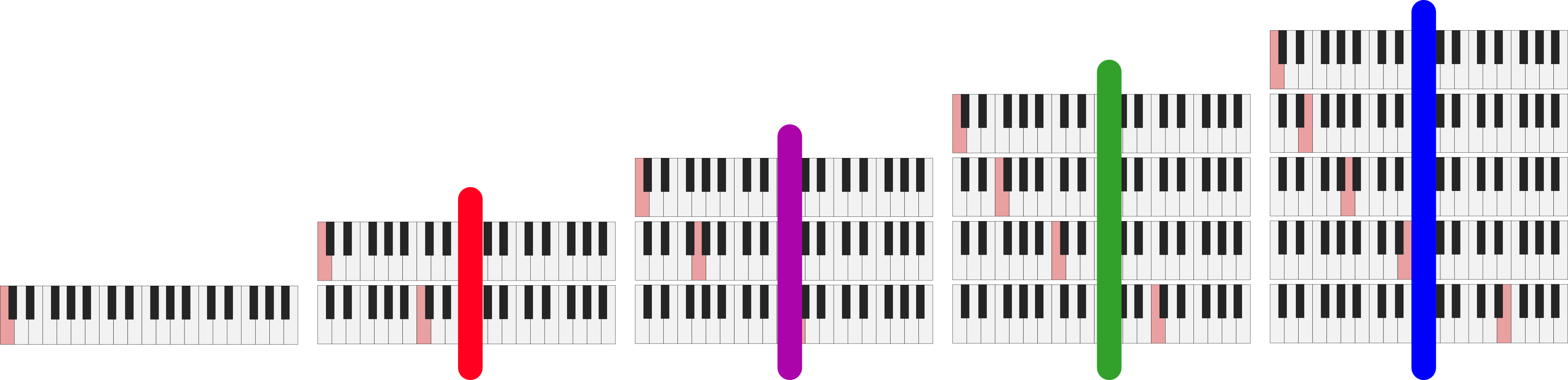
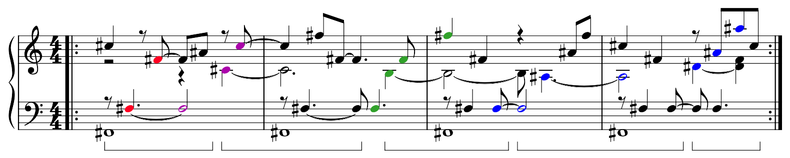
We add in notes to the piece in an order determined by flattening the grid. We traverse the columns from left to right, ignoring duplicate notes, as follows:
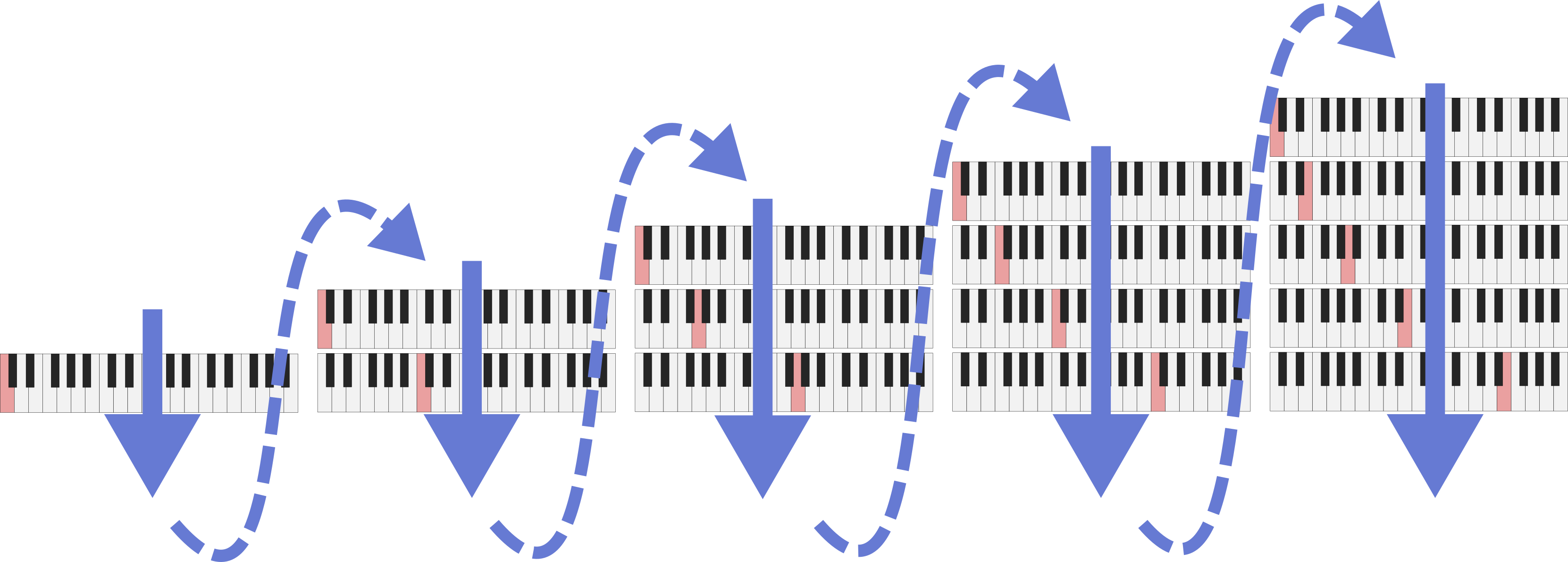
Procedure for flattening the overtone grid
Notes are introduced in this order. While there many repeated notes, there are 10 unique notes. We can see the introduction of each new note by looking at the score where the new note introductions are highlighted:
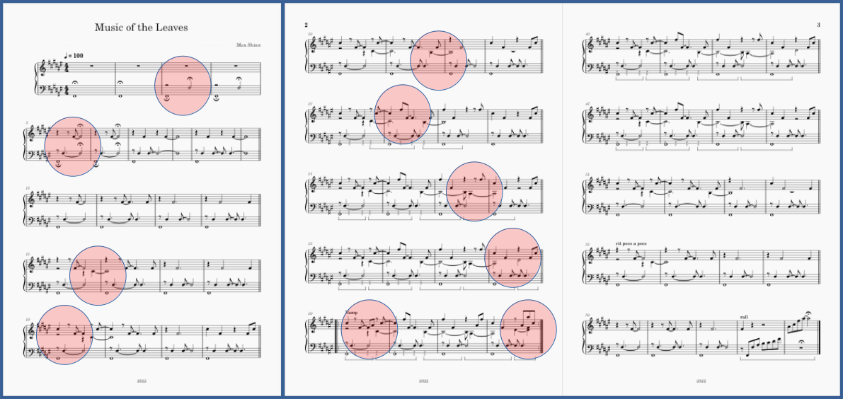
Highlighted positions indicate where a new note in the flattened overtone grid is introduced in the score.
We also can hear each new note in the recording, see a new unique set of stripes show up in the spectrogram of the recording when a new note is introduced.
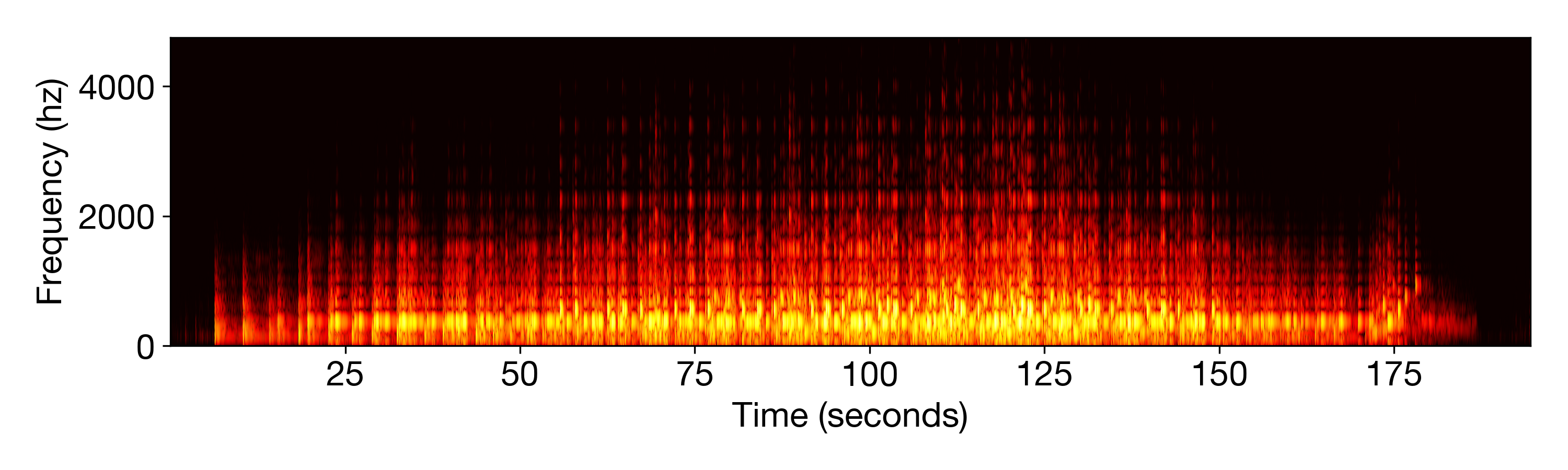
Spectrogram of the recording of Music of the Leaves.
So, the structure is made up of a flattened version of the overtone grid, and the notes come from patterns obtained by traversing the grid in different directions.
Appendix: Patterns on the grid
There are several patterns to the overtone grid. First, notice that the bottom row is the overtone series. This is because the bottom row is where \(M=1\), so \(M/N\) is the same as \(1/N\).
But interestingly, the second row from the bottom also appears to form an overtone series, but missing the first note. If we try to extrapolate it out, we see that it would be exactly one octave lower. Mathematically, this is because if we replace \(L\) with \((2L)\) (i.e., the string length for the tone one octave lower), then \((2L)/1\), \((2L)/2\), \((2L)/3\), and so on is just the overtone series for a string of length \(2L\)!
This same trend continues as we go to higher rows. In the third row from the bottom, we have the top of an overtone series which starts on the low F, corresponding to a string of length \(3L\). It becomes more difficult to notice after the third row, but the trend still continues. This row structure comes directly from the mathematical definition of the overtone series.
The columns are even more interesting, giving rise to a reverse of the overtone series, the “undertone series”. In the normal overtone series, we start with the fundamental frequency, and then go up an octave, and then a perfect 5th, then a perfect 4th, then a major 3rd, and so on. In the columns, we do the opposite. Our “pseudo-fundamental” frequency occurs on a high note at the bottom of the column. As we travel upwards in the grid, we first go down an octave, and then down a perfect 5th, then down a perfect 4th, then a major 3rd, and so on.
There is also an interesting pattern in the diagonals. Along each diagonal, the pitch gets closer and closer to the fundamental frequency at different speeds. The main diagonal corresponds to the case where \(M=N\), and thus, \(M/N=1\), so this will always be the value of the fundamental frequency. But what about the off-diagonals? The first diagonal is defined as the combinations of \(M\) and \(N\) such that \(M-N=1\). So then, we have \(L\times 2/3\), \(L\times 3/4\), \(L\times 4/5\), and so on. As the value of \(N\) gets larger, we will get closer and closer to the fundamental frequency.
Acknowledgement
Music of the Leaves was based on a conversation 10+ years ago with my former research advisor Clarence Lehman. Thank you to Chiara Naldi for recording Music of the Leaves and including it in her concert series.
Code/Data:
Does “Flight of the Bumblebee” resemble bumblebee flight?
Flight of the Bumblebee is one of the rare pieces of classical music which, through its association with bees, has cemented its place in pop culture. However, it is unclear whether its composer, Nikolai Rimsky-Korsakov, actually took inspiration from bumblebee flight patterns. I address this question using new tools from ethology, mathematics, and music theory. Surprisingly, the melody line of ``Flight of the Bumblebee’’ mimics a distinctive property of bumblebee flight, a property which was not formally discovered until decades after Rimsky-Korsakov’s death. Therefore, yes, it is very likely1 that Rimsky-Korsakov observed and incorporated actual bumblebee flight patterns into his music.
In what follows, I assume the reader has a knowledge of high school level mathematics and basic music theory (chord changes, intervals, scales, etc.). This post is based on my recent preprint, available on SocArXiv.
Historical background
The piece we now call “Flight of the Bumblebee” actually comes from one of Rimsky-Korsakov’s operas, “The Tale of Tsar Saltan”. The opera is based on a story by Alexander Pushkin, which is in turn based on several folk tales. The hero, Prince Gvidon, is cast on a remote island by his jealous aunts. While there, he unknowingly saves a Swan Princess from death, so in return, she looks after his well-being. To help him to see his father again, she temporarily transforms him into a bee2 so he may fly back to the kingdom (and sting his aunts). Eventually, when he is a human again, Prince Gvidon is reunited with his father and marries the swan princess.
Flight of the Bumblebee begins towards the end of the first scene of Act III after Prince Gvidon is transformed into a bee. The first half of the piece serves as background music for the Swan Princess’ singing as Prince Gvidon flies away. The second half serves as a transition from the first to second scene of Act III. In most renditions of this piece today, the Swan Princess’ vocal line is removed. The piece introduces the “bumblebee” theme, which continues to be a central theme of Act III as Prince Gvidon flies around the court causing mischief.
Despite the fact that Flight of the Bumblebee is by far the most recognisable piece of music Rimsky-Korsakov wrote in his lifetime, he didn’t consider it to be one of his major works. In fact, Rimsky-Korsakov didn’t even include it in his own suite of highlights from the opera3. This piece was relatively unknown until 1936, when it first4 entered pop culture as the theme song for the radio show “The Green Hornet”. It only took a few years to become widely recognisable, in large part due to a 1941 big band jazz cover by Harry James.
Bumblebee flight
In accordance with the cliché “busy as a bee”, bumblebees spend most of their day looking for food. So, we can understand bumblebee flight patterns by understanding how they forage for food. New miniature radar technology allows us to track the flight of foraging bumblebees. One important characteristic aspect we have discovered about insect foraging flight patterns, and bumblebee flight in particular, is the presence of lots of short movements and a few very large movements. At any given point in time, a bee may choose to move in any direction it wants. Most of the time, it will move a small distance. However, sometimes, it will make very large movements. For example, it may travel long distances and then carefully explore a small patch. Relatively speaking, bees will make fewer moderate-sized movements: most movements will be very small, but those which aren’t small will be very large. This has been shown to be optimal behaviour for bumblebees in many situations. In fact, algorithms inspired by this bumblebee behaviour have been used to tackle complex engineering challenges. This type of movement is in contrast to, e.g., the movement of spores released from trees, which tend to drift gently with the wind and not make large, sudden movements across a pasture. We will refer to these large movements as “jumps”.
If you think about it, it makes sense why bees might prefer to sometimes make very large movements when they are searching for food. If they always take small steps, they may never get to the large food source that is on the other side of the meadow. Indeed, this strategy is used by a wide range of animals beyond bumblebees5.
Mathematical analysis of bumblebee flight
To represent these flight patterns, we need to build an extremely simple model which is easy to work with and can be applied to a melody line. First, we need a way to relate the notes in a melody line to the location of a bee. One natural way is to assume that the ups and downs of the melody line correspond to movements of the bee. We can do this by assigning a numerical value to each note in the melody line, where 0 is the lowest note on the piano keyboard and each half step interval is 1 higher than the previous. Then, tracking the note in the melody line is the same as tracking the location of the bee. With this representation, a small movement for a bee is equivalent to a small interval in the melody line. Likewise, a “jump” for the bee is analogous to a “jump” in the melody line, or a large interval.
Now we can think about how a simple bumblebee flight model might operate. The “small steps and large jumps” behaviour we described in the previous section depends only on the sizes of the steps the bee takes at subsequent points in time, not on the direction. So without making assumptions about the direction of each step, we can specify the probability of having steps of different sizes. Then, we can assume that the bee goes in a random direction at each step. This model, known as a random walk, is used to model a huge number of phenomena in the natural world.
We will compare two models for choosing our step sizes in the random walk6. The first, the “geometric” model, is a good representation for most types of data. It posits that steps become proportionally less frequent as they get larger. So, if 50% of steps are of size 1, 25% will be of size 2, 12.5% will be of size 3, and so on. This means that large step sizes are extremely infrequent: if we continue the pattern forward, a step size of one octave (12) will only occur once every 4000 steps, and a step of two octaves (24) will occur once every 16 million steps!
By contrast, we can also use a “powerlaw” model for step sizes. Here, the probability of having a step of a given size is proportional to a power of the size of the step. This is harder to do in our head, so I worked out these numbers for us: if 50% of steps are of size 1, then only 15% of steps are of size 2, and 7% are of size 3. But, if we go out to larger steps, a one-octave jump will occur once every 146 steps, and a two octave jump will occur once every 485 steps! So, compared to the geometric model, the powerlaw model allows large jumps to happen much more frequently, with relatively fewer medium-sized jumps. Both of these models have only one parameter, describing the scale on which they operate.
Here is a simulation of what a bumblebee’s flight path might be under each model.
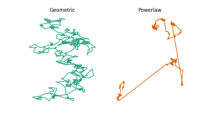
Example 2-dimensional flight trajectories from a geometric or powerlaw random walk model.
As you can see, the powerlaw model involves several large jumps, whereas the geometric model doesn’t. You can compare this to some example bumblebee flight trajectories measured by Juliet Osborne and colleagues, which show patterns which more closely resemble the powerlaw model than the geometric model.
While bumblebees fly in three dimensions, our melody line is only measured in one dimension. So, we need to convert these models into one dimension in order to compare them to Flight of the Bumblebee. First, let’s simulate these models and compare them to the actual melody line. These simulations try to match the qualitative character of the jumps of the melody line, rather than the exact “flight path” of the melody line. Here are example flight paths from the one-dimensional versions of these models, as well as the one derived from the melody of Flight of the Bumblebee:
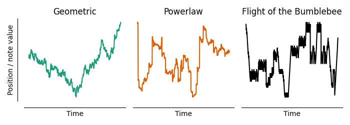
Example 1-dimensional “flight” trajectories from a geometric or powerlaw random walk model, compared to the melody line from Flight of the Bumblebee.
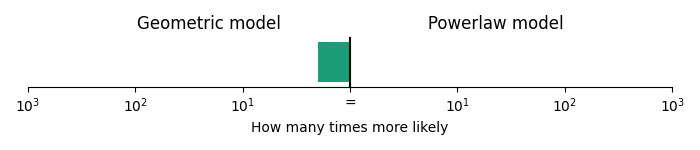
The melody line appears to have a more similar “jumpiness” to the powerlaw model than the geometric model. We can formalise this by fitting the models directly to the jump sizes in melody line (through maximum likelihood, see the appendix on methods for details), and then evaluating the fit to see which model is more likely given the data. When we do so, we find that the powerlaw model is \(1.5 \times 10^{72}\) times more likely than the geometric model!
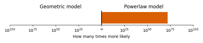
Comparison of geometric and powerlaw model.
This gives us very, very strong evidence that the Flight of the Bumblebee follows a pattern involving small steps and large jumps, over a pattern with a more balanced distribution of small and medium sized jumps.
Control analysis
Flight of the Bumblebee is based on the chromatic scale, and the chromatic scale contains lots of small intervals. Is it possible that this correspondence to the powerlaw model is just due to the extensive use of the chromatic scale? To test this, we can perform the same analysis on the other7 highly-chromatic piece of classical music widely known in pop culture: Entry of the Gladiators by Fučík (i.e., the circus song). Entry of the Gladiators also contains lots of chromatic passages and several large jumps. However, in stark contrast to Flight of the Bumblebee, given the melody line in Entry of the Gladiators, the geometric model was 1.8 times more likely than the powerlaw model.
Comparison of geometric and powerlaw model on Entry of the Gladiators.
This means that not all music based on the chromatic scale follows powerlaw step sizes.
At first, it may come as a surprise that Entry of the Gladiators isn’t better fit by powerlaw model. Like Flight of the Bumblebee, it also has lots of small intervals and lots of large jumps. In fact, it has far more large jumps than Flight of the Bumblebee. The reason it is not better fit is because Entry of the Gladiators also contains several intermediate-sized jumps. These intermediate-sized jumps aren’t predicted by the powerlaw model or by models of bumblebee flight. Flight of the Bumblebee contains almost exclusively chromatic steps and large jumps, which makes the powerlaw model a better fit. This means that Flight of the Bumblebee bears more of a mathematical resemblance to the behavioural patterns of bumblebee flight than this other highly-chromatic piece.
What did Rimsky-Korsakov intend to write?
These analyses raise an important question: is there a music theory explanation for including large jumps beyond the imagery of bumblebee flight? Likewise, which aspects of the piece are intended to invoke the imagery and which are incorporated for other musical or artistic purposes?
We know that Rimsky-Korsakov didn’t explicitly implement these mathematical models in his music. Not only was there scarce knowledge about insect behaviour when the Tale of Tsar Saltan premiered in November 1900, but the mathematics on which the models are based hadn’t even been invented yet! In order to make a judgement about step sizes in the melody line, we first must understand what musical and artistic aspects influenced the melody line. Let’s explore two here: the hero’s main theme, and the use of the whole-tone scale.
Hero’s main theme
One important component of the melody line is the hero Prince Gvidon’s theme8 (leitmotif) within the opera. This theme comes from the folksong “Заинька Попляши” (“Zainka Poplyashi”, which roughly translates to “Dance, bunny, dance!”), a song with which Rimsky-Korsakov was intimately familiar. The theme is:
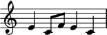
Leitmotif of Prince Gvidon’s.
As you can see below, the character’s theme is clearly represented in main bumblebee melody line, as indicated by red note heads:
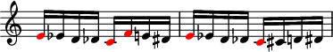
Melody line of Flight of the Bumblebee with highlighted leitmotif.
What this means is that one of the most common jumps, the jump of a perfect 4th in the main theme, can be “explained” by this theme. Since the frequency and size of jumps is critical in our mathematical analysis, we can repeat the analysis while ignoring these specific jumps in the melody line. As we see, doing so doesn’t ruin the mathematical effect described in the previous section: the powerlaw model is \(1.8 \times 10^{65}\) times more likely, given the melody line.
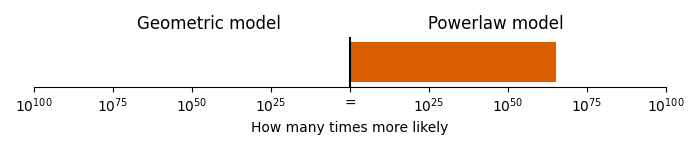
Comparison of geometric and powerlaw model.
So, the use of perfect 4th jumps to capture Gvidon’s leitmotif isn’t a major factor in what makes this melody resemble bumblebee flight.
Whole-tone scale
The piece also has a close connection with the whole-tone scale. While the whole-tone scale is most closely associated today with the French impressionists like Debussy and Ravel, it was actually used much earlier by Rimsky-Korsakov’s contemporaries as a building block of Russian nationalistic music. In this school of music, the whole-tone scale is used to represent the magical, the regal, the ominous, and the surreal.
Given the magical nature of a human transforming into a bumblebee, it may come as no surprise that the whole-tone scale plays a prominent role in Flight of the Bumblebee. Recall that there are only two whole-tone scales, which contain no notes in common.
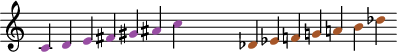
The two whole-tone scales.
Since the scales contain no notes in common, we can classify any given note as belonging to one of the two whole-tone scales.
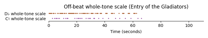
In Flight of the Bumblebee, almost all of the pitches on the eighth note beats fall into the C♮ whole-tone scale, and all of the notes on the off-beats fall into the D♭ whole-tone scale. This trend is only violated five times. In three cases, the piece modulates from A minor to D minor (the subdominant), when the whole-tone scales switch. One violation is to make the melody line align properly at the repeat9, and the final violation is to make sure the final note of the piece falls on A, the tonic.
We can visualise this by plotting each on-beat in the melody line of the piece. The x axis indicates the time at which each note is played, and the y axis indicates which whole-tone scale the note comes from. If we show the entire piece in one plot, the on-beats look like this:
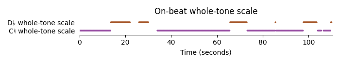
The whole-tone scale associated with each on-beat in Flight of the Bumblebee. Individual points appear as lines because they are very close together in time.
And the off-beats look like this:
The whole-tone scale associated with each off-beat in Flight of the Bumblebee. Individual points appear as lines because they are very close together in time.
There aren’t very many switches between whole-tone scales, and those that do occur have a clear musical purpose. This appears to be a deliberate use of the whole-tone scale in the piece.
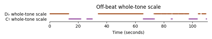
An objection one might make to this is that the whole-tone scale is by necessity connected with the chromatic scale. Since Flight of the Bumblebee uses the chromatic scale, this property of the whole-tone scale might arise naturally.
To show this objection doesn’t apply, we can perform the same analysis on Entry of the Gladiators. Here, unlike in Flight of the Bumblebee, we see no deliberate use of whole-tone scale for the on-beats:
The whole-tone scale associated with each on-beat in Entry of the Gladiators.
Or for off-beats:
The whole-tone scale associated with each off-beat in Entry of the Gladiators.
This means that the whole-tone scale seems to have been deliberately used by Rimsky-Korsakov, but not by Fučík, in constructing the melody line.
Interestingly, this pattern makes it more “difficult” to write a melody line which includes large jumps. This is because large jumps can only be included if they sound nice. It is musically “easy” to maintain the whole-tone scale pattern while making medium-sized jumps, because most medium-sized jumps sound pleasant in many different contexts. All intervals from minor 2nds to major 6ths are extremely common across a wide range of musical genres. By contrast, it is more difficult to make large jumps sound nice. In most pieces, large jumps often occur at octave, 9th, 10th, or flat 7th intervals, all of which would violate the alternating whole-tone scale pattern. This means that the use of the whole-tone scale in the melody line actually makes it more difficult to have large jumps. So, because of the whole-tone scale pattern, the presence of large jumps in Flight of the Bumblebee is even more surprising than the mathematical analysis suggests.
Rimsky-Korsakov also left out some medium-sized jumps which fit the whole-tone scale pattern. Another “valid” jump under the whole-tone pattern, and one which is extremely common in other pieces, is the perfect 5th. However, the perfect 5th, a medium-sized jump, only occurs once in the melody line of Flight of the Bumblebee. Two similarly “easy-to-use” intervals which satisfy the whole-tone pattern, the minor 3rd and the major 6th, don’t occur at all. The only medium-sized interval that Rimsky-Korsakov uses is the perfect 4th, which we already showed was a result of Prince Gvidon’s theme. So, the use of large jumps and not medium sized jumps appears to be a deliberate choice by the composer.
Conclusion
Flight of the Bumblebee is a much more musically complex piece than it initially seems. Rimsky-Korsakov appears to have deliberately mimicked an important property of bumblebee flight within his music. Mathematical models to describe bumblebee flight, invented long after Rimsky-Korsakov’s time, end up providing an excellent fit to his melody line. On top of this, he incorporated interesting features from a music theory perspective, including the main character’s theme and a whole-tone scale pattern. These musical features don’t explain the melody line’s resemblance to bumblebee flight. While we will never know if Rimsky-Korsakov actually observed bumblebee flight while composing Flight of the Bumblebee, it sure is fun to speculate10, isn’t it?
Appendix: Methods
To find the melodic pattern, I downloaded Nicolas Froment’s engraving of the Rachmaninoff piano arrangement and cut out everything except the melody line. Then, I cross-referenced this to the score from the original opera, page 262-267, to tweak the melody line to ensure it is faithful to that of the opera rather than the piano arrangement, correcting for octaves, breaks, repeats, etc. I exported this as MIDI (attached below) and analysed it using a Python script (attached below). Likewise, I used James Birgham’s engraving of the piano reduction of Entry of the Gladiators and exported to MIDI (attached).
I only used sections of Flight of the Bumblebee which were part of the rapid, recognisable melody, concatenating across breaks. Likewise, I excluded the trio section of Entry of the Gladiators since it isn’t based on chromatics. Repeated notes were excluded since a jump of zero in a discrete random walk doesn’t correspond to any kind of step in a continuous Wiener or Levy process. I adjusted the octave down in two cases (penalising the powerlaw model): once for a two-octave jump in the final run of Flight of the Bumblebee, since it was an artistic flourish for the finale; and once for a two-octave jump when the melody line switches from treble to bass in Entry of the Gladiators.
Model fitting was performed by finding the pairwise distances between neighbouring points in each timeseries, and then fitting the counts of each to a geometric or Zipf distribution through maximum likelihood. A numerical minimisation routine was used to find parameters which maximised the likelihood function.
The music theory analysis was partially my own (whole-tone scale analysis) and partially based on work from Rosa Newmarch, Victoria Williams and John Nelson (historical and motivic analysis). Thank you to Sophie Westacott for helpful comments, and to the giant bumblebee who regularly hovers outside my window and then darts away for inspiration.
Code/Data:
- Analysis script
- Script to generate plots
- Flight of the Bumblebee MIDI melody
- Entry of the Gladiators MIDI melody
Footnotes
-
contrary to Betteridge’s law ↩
-
In the Pushkin story, he was also transformed into a mosquito and a fly to see his father and sting his aunts, for a total of three trips back. ↩
-
Due to the piece’s broad recognisability today, many orchestras insert Flight of the Bumblebee into the suite anyway. ↩
-
Contrary to claims from some sources, it didn’t appear in Charlie Chaplin’s 1925 film “Gold Rush” - instead, it appeared in the 1942 version, which used different music. ↩
-
Similarly, when humans seek food, it is occasionally wise to take a large step and go to the supermarket instead of always looking inside the refrigerator. ↩
-
As a technical note: ideally, we would want to consider the difference between a Wiener process (Brownian motion) and a Levy process, which is similar to Brownian motion except the steps are powerlaw-distributed. Since our melody line is discrete in pitch (i.e. there are only 12 notes per octave), we must use a model with discrete steps in order to get a likelihood which makes sense. So, we use the geometric distribution and the discrete powerlaw distribution (zeta or Zipf distribution). We use the geometric distribution as a stand-in for the normal distribution, since there is no well-known discrete half-normal–like distribution with support on all the natural numbers. ↩
-
The use of “the” was deliberate. I don’t think there are any other pieces of classical music which are widely known in pop culture and rely so heavily on chromatics. The internet doesn’t seem to think so either, but please correct me if I am wrong! (Habanera from Carmen doesn’t count, since it only embeds a descending chromatic scale within a surrounding not-so-chromatic melody.) ↩
-
Prince Gvidon has two main leitmotifs in the opera, but only the one shown here participates in the melody line. The other one also appears in Flight of the Bumblebee but not within the melody line: it is the descending and ascending staccato line which appears several times in the accompaniment. ↩
-
The repeat is only found in the original opera score, not in the popular piano reduction. ↩
-
Speaking of speculation, here is a pretty big leap: Rimsky-Korsakov is known to have had synesthesia, associating colours with different keys. While there is no documented evidence of Rimsky-Korsakov’s associations with the minor keys, there are descriptions of his associations with the major keys. While I was unable to find the primary source describing Rimsky-Korsakov’s colour-key synesthesia, I do believe there to be a primary source in Russian, because several of the secondary sources use different translations of the colour names.
The parallel and relative major keys actually line up well with bumblebees. Flight of the Bumblebee is written in A minor, and modulates to D and G minor. In Rimsky-Korsakov’s classification, the parallel major keys, A, D, and G major, correspond to rose, yellow and gold, respectively. These colours evoke the imagery of a yellow-gold bumblebee flying to bright flowers. Additionally, the relative major keys of these minor keys—C major, F major, and Bb major—correspond to green and white, with no documented correspondance for Bb major. These associations, while interesting, are probably a coincidence, especially without evidence about his colour associations with the minor keys. ↩
Are buffets efficient?
I recently attended an academic conference and was struck by the inefficiency of the buffet-style dinner. The conference had approximately 500 attendees, and dinner was scheduled for 6:30 PM following a 15 minute break in the conference program. A 15 minute break is not enough time to go back to the hotel room and take a nap, and barely enough time to find a quiet corner and get some work done, but it is a perfect amount of time to crowd around the buffet waiting for dinner to open.
When dinner finally opened, all of the food was arranged on a single table, inviting the attendees to form a single line to serve themselves. As you can imagine, this line was quite long. I was lucky enough to be one of the first people through the line, but by the time I finished eating a half hour later, the line was still very long. I had been waiting for someone who was towards the middle to end of the line, and this person still had not made it through yet.
I found it odd that feeding people should be so slow. From my experiences in undergraduate dining halls, it is possible to feed more people in a shorter amount of time. A key difference between these situations is that in undergraduate dining halls, food is often served at individual stations, meaning you only need to wait in line for food you want to eat. By contrast, in the catering style, it is often served all at one table, with diners waiting in a single line and accessing the dishes one by one. I wanted to examine the efficiency of these two systems. This is important not only for minimizing the mean wait time so that everyone gets their food faster, but also for minimizing inequality between people at the front and end of the line. This ensures that everyone has the opportunity to dine together.
Model
I modeled this situation as a single line in a buffet versus individual lines for each different dish. I made the following assumptions:
- Some people may be faster or slower at serving themselves.
- Some foods can be served faster than other foods.
- People may not want all of the food which is being served, and each person wants a different random selection of foods.
- Only one person can serve themself a particular dish at one time.
- When dishes have their own individual lines, people look at the lines for the foods they want to eat and stand in the shortest line next.
- People already know what the options are and where they are located.
I calculated the wait time for each person in the simulation as the total amount of time it took a person to pass through the buffet. I then looked at the mean wait time for the group as well as the inequality in wait time for people in the group, defined as the third quartile minus the first quartile. Each simulation was run many times to ensure accurate statistics.
Number of dishes wanted
Let us suppose that not everyone wants the same number of dishes, but that all dishes are equally attractive. First we look at the case when there are a limited number of dishes.
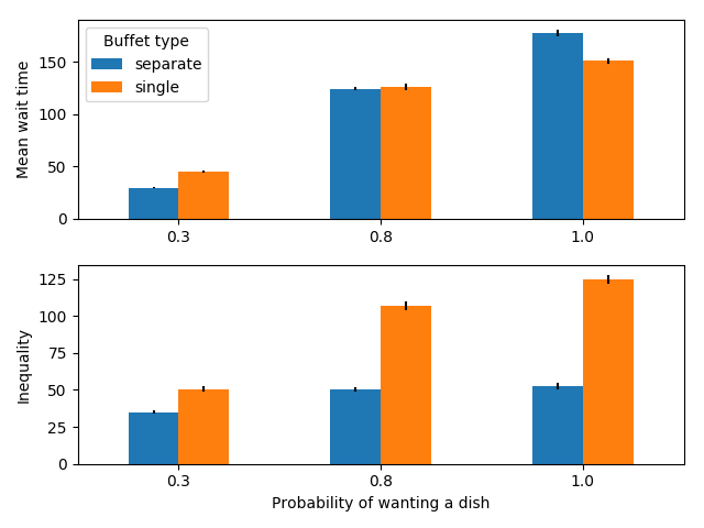
100 people serving themselves in a buffet with 6 dishes
We see that when there aren’t very many dishes and most people want all of them, it is faster to have a single line. This may be counter-intuitive, but it is due to the fact that people do not optimally distribute themselves, but instead choose the shortest line. Suppose for example that one dish is much slower to serve than all of the others. People who choose this food last will have to wait approximately the same amount of time as they would have if there was a single line and they ended up at the end, because this dish serves as the bottleneck. However, the people who are at the front of this line will still need to wait in more lines for the other dishes, because other people tried to serve themselves these dishes first. As a result, having multiple lines can sometimes increase the amount of time for the fastest people and not decrease the amount of time for the slowest people.
Additionally, there is a large inequality in wait times, i.e. some people will get through the line quickly, while others will be stuck in line for a long time. This is the case for both serving styles, but is especially pronounced for the case with multiple lines.
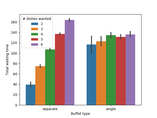
Let us also examine the case when there are many dishes to choose from.
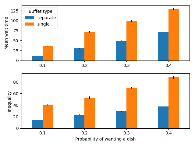
100 people serving themselves in a buffet with 20 dishes
When there are many dishes to choose from (here 20), no matter how many dishes people may want (within reason), individual lines reduce both the mean wait time and the inequality in wait times compared to a single line. Intuitively, this is because people can distribute themselves and they only have to wait for the dishes they want to eat.
Additionally, let’s look at the case when there are many people.
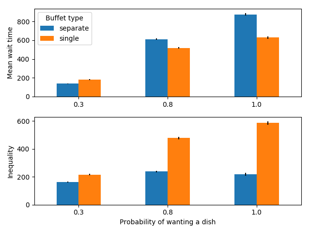
500 people serving themselves in a buffet with 6 dishes
In this case, we see the counter-intuitive result again: the mean wait time is quite a bit higher for individual lines when most people want most of the foods, however inequality is still lower.
Finally, we can examine the case when there are very few people.
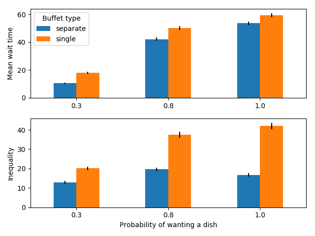
30 people serving themselves in a buffet with 6 dishes
In this case, separate lines are better for both mean wait time and equality.
Fairness
A fair system is one in which the amount of time someone waits is proportional to the number of dishes they want. In an unfair scenario, someone who only wants one dish must wait for the same amount of time as someone who wants all of the dishes.
Let’s look at whether this form of fairness holds. First, we look at how long someone must wait depending on how many dishes they want.
Average wait time differs depending on how many dishes a person would like
As expected, when there is only one line, everyone must wait for approximately the same amount of time, no matter how much food they want to eat. People who want all of the dishes in a line must wait for less time on average, but someone who only wants one dish must wait for a very long time. By contrast, when there are multiple lines, the amount of time people wait is proportional to the number of dishes they want to try.
Similarly, it might be fairer that someone who can serve themself quickly has a shorter waiting time than someone who is slower.
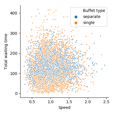
Points represent people. There is no significant correlation (\(p>.2\)) between time spent waiting and serving speed
Unfortunately this does not seem to be the case in either system. Rather, people who are slow to serve themselves take approximately the same amount of time in line as those who are fast.
Summary and conclusions
In summary, when there are a lot of people present, if everyone wants most of the food at the buffet, a single line counter-intuitively reduces the mean wait time. However, this single line substantially increases inequality in wait times, meaning that some people will have to wait for a long time while others can go through immediately. Additionally, people who only want a small amount of food must wait a long time to serve themselves. A more fair but slightly less efficient system is one where there is a separate station for each dish, but this can be inefficient when most people want most of the dishes available.
This analysis leaves out a few factors which are difficult to account for. For example, it assumes the amount of time taken to walk from one food to another is negligible, and that people know a priori what food they would like to eat and where it is located. Both of these have the potential to slow down serving times in the case with separate lines. This analysis also doesn’t account for several other factors which are important in real life. For example, it assumes that space is not an issue. It also assumes there is enough seating to accommodate everybody; if only a limited amount of seating is available, a high inequality is desirable as it prevents everyone from going to the dining area at one time.
One method which is often employed to speed up single lines is having more than one identical line, or two sides on the same line, likewise, in the case of separate lines, there are sometimes “stations” which have identical dishes. In both cases, because we assume people balance themselves by going to the shortest line, doubling the number of copies of all dishes would be expected to approximately cut the mean wait time in half.
Code/Data:
Optimality in card shuffling
Many powerful minds have devoted countless decades to the academic study of card games. However, relatively little attention has been given to the best way to shuffle a deck of cards. There are several different methods that people have developed to shuffle cards:
- The riffle shuffle: The classic shuffling method. Cut the deck approximately in half. Take one half in each hand, and let the cards from both decks fall on top of one another.
- The overhand shuffle: Another very popular method. Hold the cards in one hand, and take the cards with your other hand, and let them fall on top.
- The Hindu shuffle: A method popular in India. It is a different style of performing an overhand shuffle.
- The pile shuffle: Create several sub-decks of cards, by placing cards one-by-one into a (potentially random) sub-deck. Then, combine the sub-decks together.
It has been claimed that seven, eight, or more riffle shuffles are necessary to obtain complete randomization. However, these studies assume that any difference in probability between a shuffled deck and a fully random permutation can be exploited by the players. This is an important model for casinos where large amounts of money are at stake, but for games between friends where perfect randomness is not needed, seven or eight shuffles in between hands causes a substantial delay in the game.
Thus, below I describe how many shuffles you need in practice instead of in theory. My evaluation looks for patterns and irregularities in hands that would be dealt. It accounts for three types of patterns—suits, ranks, and clusters/straights—by looking at the joint distribution of of these frequencies compared to a null distribution. (For instance, a six card hand containing four of one suit and two of another is highly unlikely.) I simulate a number of different shuffling methods and find the probability of obtaining the arrangements generated by these shuffles in a truly random deck.
Each of the shuffles starts with either fully ordered decks (i.e. a new deck of cards), or else with cards in an order representative of a specific card game. I compare these to a deck which started out fully randomized before the shuffle as a control, which is therefore guaranteed to be fully randomized after the shuffle. All shuffles should be compared to the randomized deck, i.e. the red line in the plots.
Card game deck patterns used in all figures which follow.
Riffle shuffle
The riffle shuffle is arguably the most popular shuffling method. The standard accepted mathematical model for the Riffle shuffle is called the Gilbert-Shannon-Reeds model (GSR model). (Yes, that’s Claude Shannon.) This model assumes that the shuffler is an expert and can dynamically adjust the rate at which cards are laid down from each hand during the shuffle. It states that the probability of putting down a card from either hand is proportional to the relative size of the deck in that hand. For example, if your left hand had 30 cards and your right hand had 10, you would have a 3/4 probability of the next card coming from your left hand.
Hesitant to accept this definition, I developed another model which includes a skill parameter \(\lambda\). High \(\lambda\) means that there is a low probability of two consecutive cards being dealt from the same hand, whereas low \(\lambda\) means there will be large bunches of cards from the same hand in the deck. This is motivated by the fact that, given the speed at which cards are shuffled, most people do not have the reaction time necessary to adjust the rate at which they let cards fall from either hand, and also by the fact that casino dealers come close to alternating cards from each hand.
In order to test these models, I collected data from my own shuffles to determine the most likely model. I found that my model was slightly more likely given the data, but if you account for the fact that my model has a parameter whereas the GSR model has none, the GSR model is a slightly better fit to the data.
Because they were close, I decided to test both cases, and also to vary the skill level \(\lambda\). I tested four cases: a novice shuffler (\(\lambda=0.3\)), an average shuffler (\(\lambda=0.45\), the best fit to my shuffling data), an expert shuffler (\(\lambda=0.8\)), and the ideal GSR case (which has no parameter).
Effectiveness of riffle shuffles as a function of the number of consecutive shuffles.
As we can see, people comfortable with a riffle shuffle need approximately 4 shuffles in order to randomize the deck, which is approximately half of the theoretical recommendation. An average card player does not have any advantage over a professional casino dealer in this regard. Of course, if you’re not riffle shuffling very well, it will take far more shuffles to achieve the same degree of randomness.
Overhand/Hindu shuffle
The overhand shuffle is equivalent to dividing the deck into a number of sub-decks and then recombining those decks in reverse order. By watching several YouTube videos of people performing the overhand shuffle, there is a wide variety in the number of times people will divide the deck when performing the shuffle. Most people do it around 5 times, but some people consistently do more or fewer than this.
Here, we consider the cases of 5 cuts, 3 cuts, and 8 cuts, as these values covers the typical range of cuts.
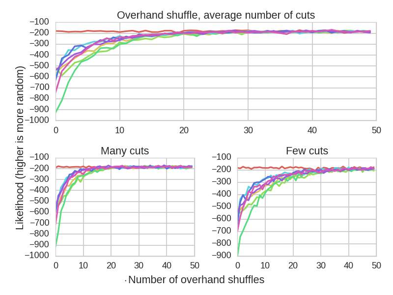
Effectiveness of overhand shuffles as a function of the number of consecutive shuffles.
It takes many more overhand shuffles to randomize the deck. Assuming an average number of cuts, it takes approximately 25 shuffles, which is 20-60 times less than the theoretical result. When you only cut the deck 3 times during an overhand shuffle, this number jumps to almost 40. Nevertheless, this goes against the theoretical finding, and suggests that the overhand shuffle is a valid and useful method, even if it is a bit more time consuming.
Pile shuffle
The pile shuffle has many variants. In the strict form, the shuffler deals all of the cards into some number of piles, and then stacks the cards on top of each other.
Clearly this strict form is both deterministic and highly patterned, and thus it is rather ineffective. Sometimes, people will add a slight bit of randomization by picking up the piles in a different order than they laid them down. More frequently, people will perform this deal by randomizing the order in which they lay down cards into the decks. Sometimes they will do so while keeping the decks approximately the same size, and sometimes they will disregard deck size. (However, note that people are notoriously bad at randomizing, so these should be considered the maximum limits of randomization rather than the method’s true amount of randomization.)
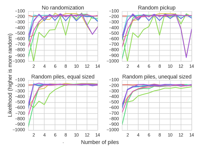
Effectiveness of pile shuffles as a function of the number of piles.
We see that pile shuffling is not very efficient when only performed once. The reason appears to be that this method does not randomize the ranks in the deck. If you started with an ordered deck, you can be nearly certain that if you pick up a 3, the next card will not be a 2. Most versions of pile shuffling are ineffective for this reason. The only version which works is the version which keeps the decks at an approximately similar size throughout the duration of the shuffle, while using at least eight decks. However, this also assumes that the shuffler is able to generate near-random numbers, which is impossible without either a random number generator or knowledge of strategies for generating random numbers without one.
Miscellaneous results
I simulated two styles of deals from the shuffled deck: one where the top 6 cards were taken from the deck, and one where there were 4 players, and 6 cards were dealt to each in a clockwise manner. Results were nearly identical for both cases, so only results for the former are included here.
I also simulated the mixed case which combines riffle shuffles and that overhand shuffles, with the hypothesis that adding a few overhand shuffles could reduce the number of riffle shuffles needed to randomize the deck. Unfortunately, this turned out to not be the case. Adding one or two overhand shuffles to different places in the riffle shuffle sequence was not able to reduce the number of riffle shuffles needed to randomize the deck.
If we assume that the riffle shuffle takes approximately 5 seconds to perform and the overhand shuffle takes 2 seconds to perform, it takes 40 seconds to randomize the deck using the overhand shuffle but 20 seconds to randomize it using the riffle shuffle. If we assume that four cards can be dealt per second and decks can be straightened and stacked at a rate of one per subpile, a suitable pile shuffle would take 21 seconds. However, this is also assuming suitable randomization, and thus, cards may not be as randomized as in the other methods.
There are other considerations in choosing the shuffling method as well; for instance, the overhand shuffle is considered to be less damaging to the cards than a riffle shuffle, which may bend the cards.
Summary
From this analysis, we have learned the following:
- The riffle shuffle is highly efficient, requiring only 4 shuffles in order to make a deck random for most practical purposes.
- When using 5 deck cuts in the overhand shuffle, about 25 shuffles are necessary to randomize the deck. While it takes longer to perform, it is equally as effective as 4 riffle shuffles after 25 iterations.
- 10 or more riffle shuffles may be required if the shuffler lacks experience.
- The pile shuffle should generally be avoided, unless using eight or more piles, distributing cards randomly, ensuring all piles are approximately the same size, and ideally finding a way to circumvent the limitations humans have in generating random numbers.
- Combining overhand shuffles with riffle shuffles does not increase randomization compared to just using riffle shuffles.