Can humans generate random numbers?
It is widely known that humans cannot generate sequences of random binary numbers (e.g. see Wagenaar (1972)). The main problem is that we see true randomness as being “less random” than it truly is.
A fun party trick (if you attend the right parties) is to have one person generate a 10-15 digit random binary number by herself, and another generate a random binary sequence using coin flips. You, using your magical abilities, can identify which one was generated with the coin.
The trick to distinguishing a human-generated sequence from a random
sequence is by finding the number of times the sequence switches
between runs of 0s and 1s. For instance, 0011 switches once, but
0101 switches three times. A truly random sequence will have a switch
probability of 50%. A human generated sequence will be greater
than 50%. To demonstrate this, I have generated two sequences
below, one by myself and one with a random number generator:
(A) 11101001011010100010
(B) 11111011001001011000
For the examples above, sequence (A) switches 13 times, and sequence (B) switches 9 times. As you can guess, sequence (A) was mine, and sequence (B) was a random number generator.
However, when there is a need to generate random numbers, is it possible for humans to use some type of procedure to quickly generate random numbers? For simplicity, let us assume that the switch probability is the only bias that people have when generating random numbers.
Can we compensate manually?
If we know that the switch probability is abnormal, it is possible (but much more difficult than you might expect) to generate a sequence which takes this into account. If you have time to sit and consider the binary sequence you have generated, this can work. It is especially effective for short sequences, but is not efficient for longer sequences. Consider the following longer sequence, which I generated myself.
1101100011011010100
1101010111101011000
0101011110101001011
0100110101011110100
1010010101010111111
This sequence is 100 digits long, and switches 62 times. A simple algorithm which will equalize the number of switches is to replace digits at the beginning of the string with zero until the desired number of switches has been obtained. For example:
0000000000000000000
0001010111101011000
0101011110101001011
0100110101011110100
1010010101010111111
But intuitively, this “feels” much less random. Why might that be? In a truly random string, not only will the switch probability be approximately 50%, but the switch probability of switching will be approximately 50%, which we will call “2nd order switching”. What exactly is 2nd order switching? Consider the truly random string:
01000011011100010000
Now, let’s generate a new binary sequence, where a 0 means that a
switch did not happen at a particular location, and a 1 means a
switch did happen at that location. This resulting sequence will be
one digit shorter than the initial sequence. Doing this to the above
sequence, we obtain
1100010110010011000
For reference, notice that the sum of these digits is equal to the total number of switches. We define the 2nd order switches as the number of switches in this sequence of switches.
We can generalize this to \(n\)‘th order switches by taking the sum of the sequence once we have recursively found the sequence of switches \(n\) times. So the number of 1st order switches is equal to the number of switches in the sequence, the 2nd order is the number of switches in the switch sequence, the number of 3rd order switches is equal to the number of switches in the switch sequence of the switch sequence, and so on.
Incredibly, in an infinitely-long truly random sequence, the
percentage of \(n\)‘th order switches will always be 50%, for all
\(n\). In other words, no matter how many times we find the
sequence of switches, we will always have about 50% of the digits be
1.
Returning to our naive algorithm, we can see why this does not mimic a random sequence. The number of 2nd order switches is only 24%. In a truly random sequence, it would be close to 50%.
Is there a better algorithm?
So what if we make a smarter algorithm? In particular, what if our algorithm is based on the very concept of switch probability? If we find the sequence of \(n\)‘th order switches, can we get a random sequence?
It would take a very long time to do this by hand, so I have written some code to do it for me. In particular, this code specifies a switch probability, and generates a sequence of arbitrary length based on this (1st order) switch probability. Then, it will also find the \(n\)‘th order switch probability.
As a first measure, we can check if high order switch probabilities eventually become approximately 50%. Below, we plot across the switch probability the average of the \(n\)‘th order difference, which is very easy to calculate for powers of 2 (see Technical Notes).
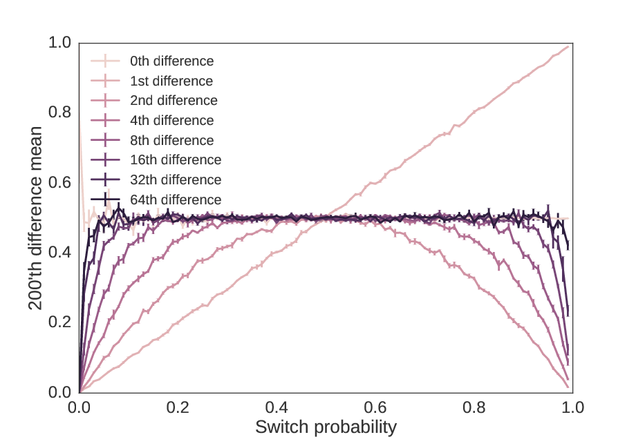
As we increase the precision by powers of two, we get sequences that have \(n\)‘th switch probabilities increasingly close to 50%, no matter what the 1st order switch probability was.
From this, it would be easy to conclude that the \(n\)‘th switch probability of a sequence approximates a random sequence as \(n → ∞\). But is this true? What if we do the powers of 2 plus one?
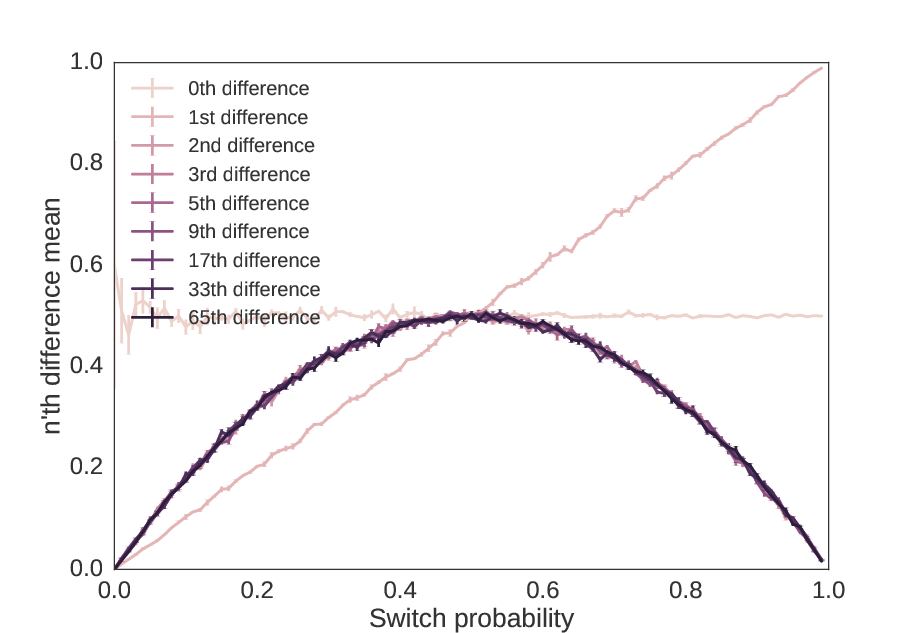
As we increase the precision by powers of two plus one, we get no closer to a random sequence than the 2nd order switch probability.
As we see, even though the switch probability approaches 50%, there is “hidden information” in the second order switch probability which makes this sequence non-random.
Is it possible?
Mathematicians have already figured out how we can turn biased coins (i.e. coins that have a \(p≠0.5\) probability of landing heads) into fair coin flips. This was famously described by Von Neumann. (While the Von Neumann procedure is not optimal, it is close, and its simplicity makes it appropriate for our purposes as a heuristic method.) To summarize this method, suppose you have a coin which comes up heads with a probability \(p≠0.5\). Then in order to obtain a random sequence, flip the coin twice. If the coins come up with the same value, discard both values. If they come up with different values, discard the second value. This takes on average \(n/(p-p^2)\) coin flips to generate a sequence of \(n\) values.
In our case, we want to correct for a biased switch probability. Thus, we must generate a sequence of random numbers, find the switches, apply this technique, and then map the switches back to the initial choices. So for example,
1011101000101011010100101000010
has switches at
110011100111110111110111100011
So converting this into pairs, we have
11 00 11 10 01 11 11 01 11 11 01 11 10 00 11
Applying the procedure, we get
1 0 0 0 1
and mapping it back, we get a random sequence of
100001
(With a bias of \(p=0.7\) in this example, the predicted length of our initial sequence of 31 was 6.5. This is a sequence of length 6.)
It is possible to recreate this precisely with a sliding window.
However, there is an easier way. In humans, the speed limiting step
is performing these calculations, not generating biased binary digits.
If we are willing to sacrifice theoretical efficiency (i.e. using as
few digits as possible) for simplicity, we can also look at our initial
sequence in chunks of 3. We then discard the sequences 101,
010, 111, and 000, but keep the most frequent digit
in the triple for the other observations, namely keeping a 0 for
001 and 100, or a 1 for 110, and 011.
(Note that this is only true because we assume an equal probability of
0 or 1 in the initial sequence. A more general choice
procedure would be a 0 if we observe 110 or 001, and
a 1 if we observe 100 or 011. However, this is more
difficult for humans to compute.) A proof that this method generates
truly random sequences is trivial.
When we apply this method to the sequences in Figures 1 and 2, we get the following, which shows both powers of two and powers of two plus one.
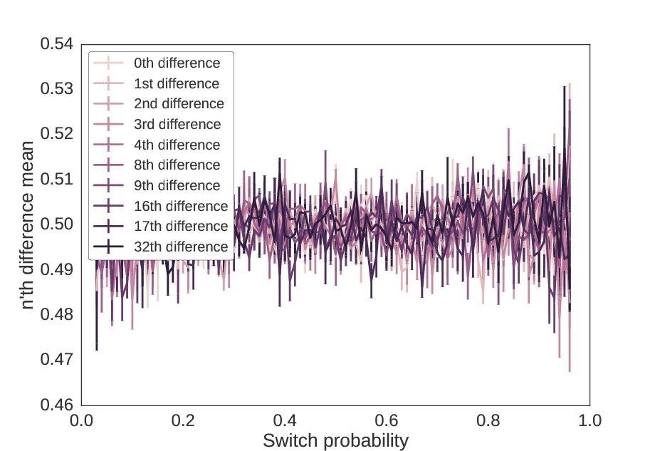
Using the triplet method, no differences of the sequence show
structure, i.e. the probability of a 0 or 1 is approximately 50%
in all differences. These values mimic those of the two previous
figures. The variance increases at the edges because the probability
of finding the triplets 010 and 101 is high when switch
probability is high, and the triplets 000 and 111 is high when
switch probability is low, so the resulting sequence is shorter.
Testing for randomness of these methods
While there are many definitions of random sequences, the normalized entropy is especially useful for our purposes. In short, normalized entropy divides the sequence into blocks of size \(k\) and looks at the probability of finding any given sequence of length \(k\). If it is a uniform probability, i.e. no block is any more likely than another block, the function gives a value of 1, but if some occur more frequently than others, it gives a value less than 1. In the extreme case where only one block appears, it gives a value of 0.
Intuitively, if we have a high switch probability, we would expect to
see the blocks 01 and 10 more frequently than 00 or 11.
Likewise, if we have a low switch probability, we would see more 00
and 11 blocks than 01 or 10. Similar relationships extend
beyond blocks of size 2. Entropy is useful for determining randomness
because it makes no assumptions about the form of the non-random
component.
As we can see below, the triplet method is identical to random, but all other methods show non-random patterns.
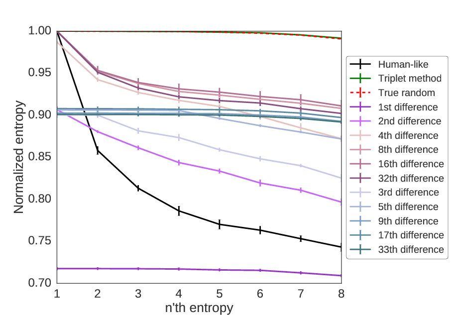
Using entropy, we can see which methods are able to mimic a random sequence. Of those we have considered here, only the triplet method is able to generate random values, as the normalized entropy is approximately equal to 1 for all sequence lengths.
Conclusions
Humans are not very effective at generating random numbers. With
random binary numbers, human-generated random numbers tend to switch
back and forth between sequences of 0s and 1s too quickly. Even
when made aware of this bias, it is difficult to compensate for it.
However, there may be ways that humans can generate sequences which
are closer to random sequences. One way is to split the sequence into
three-digit triplets, discarding the entire triplet for 000, 111,
010, and 101, and taking the most frequent number in all other
triplets. When the key non-random element is switch probability, this
creates an easy-to-compute method for generating a random binary
sequence.
Nevertheless, this triplet method relies on the assumption that the only bias humans have when generating random binary numbers is the switch probability bias. Since no data were analyzed here, it is still necessary to look into whether human-generated sequences have more non-random elements than just a change in switch probability.
More information
Technical notes
The 1st order switch sequence is also called differencing. Similarly, the sequence of \(n\)‘th order switches is equal to the \(n\)‘th difference. The 1st difference can also be thought of as a sliding XOR window, i.e. a parity sliding window of size 2.
Using the concept of a sliding XOR window raises the idea that the \(n\)‘th difference can be represented as as sliding parity window of size greater than 2. By construction, for a sequence of length \(N\), a sliding window of size \(k\) would end up producing a sequence of length \(N-k+1\). Since the \(n\)‘th difference produces a sequence of length \(N-n\), this means that a sliding window of length \(k\) would be limited to only the \((k-1)\)‘th difference.
It turns out that this can only be shown to hold for window sizes of powers of two. The proof by induction that this holds for window sizes of powers of two is a simple proof by induction. The 0th difference corresponds to a window of size 1. The parity of a single binary digit is just the digit itself. So it holds trivially in this case.
For the induction step, suppose the \((k-1)\)‘th difference is equal to the parity for a window of size \(k\) where \(k\) is a power of 2. Let \(x\) be any bit in at least the \((2k-1)\)‘th difference. Let the window of \(x\) be the appropriate window of \(2k\) digits of the original sequence which determines the value of \(x\). We need to show that the parity of the window of \(x\) is equal to the value of \(x\).
Without loss of generality, suppose the sequence of bits is of length \(2k\) (the window of \(x\)), and \(x\) is the single bit that is the \((2k-1)\)‘th difference.
Let us split the sequence in half, and apply the assumption to the first half and then to the second half separately. We notice that the parity of the parities of these halves is equal to the parity of the entire sequence. Splitting the sequence in half tells us that the first bit in the \((k-1)\)‘th difference is equal to the parity of the first half of the bits, and the second bit in the \((k-1)\)‘th difference is equal to the parity of the second half of the bits.
We can reason that these two bits would be equal iff the parity of the \(k\)‘th difference is 0, and different iff the parity of the \(k\)‘th difference is 1, because by the definition of a difference, we switch every time there is a 1 in the sequence, so an even number of switches means that the two bits would have the same parity. By applying our original assumption again, we know that if the \(k\)‘th difference is 0, then \(x\) will be 0, and if the \(k\)‘th difference is 1, \(x\) will be 1.
Therefore, \(x\) is equal to the parity of a window of size \(2k\), and hence the \((2k-1)\)‘th difference is equal to the parity of a sliding window of size \(2k\). QED.
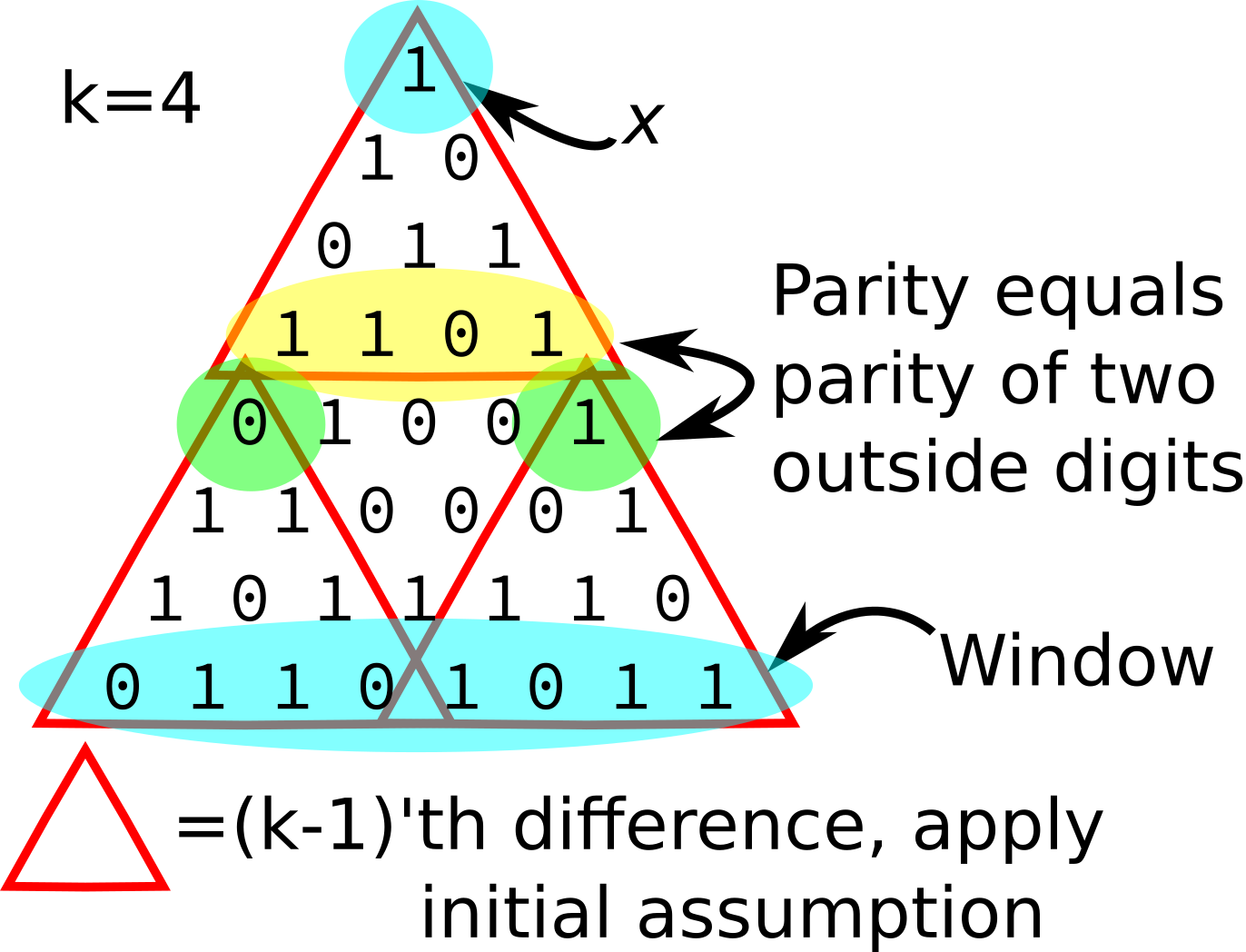
A visual version of the above proof.