Can humans generate random numbers?
It is widely known that humans cannot generate sequences of random binary numbers (e.g. see Wagenaar (1972)). The main problem is that we see true randomness as being “less random” than it truly is.
A fun party trick (if you attend the right parties) is to have one person generate a 10-15 digit random binary number by herself, and another generate a random binary sequence using coin flips. You, using your magical abilities, can identify which one was generated with the coin.
The trick to distinguishing a human-generated sequence from a random
sequence is by finding the number of times the sequence switches
between runs of 0s and 1s. For instance, 0011 switches once, but
0101 switches three times. A truly random sequence will have a switch
probability of 50%. A human generated sequence will be greater
than 50%. To demonstrate this, I have generated two sequences
below, one by myself and one with a random number generator:
(A) 11101001011010100010
(B) 11111011001001011000
For the examples above, sequence (A) switches 13 times, and sequence (B) switches 9 times. As you can guess, sequence (A) was mine, and sequence (B) was a random number generator.
However, when there is a need to generate random numbers, is it possible for humans to use some type of procedure to quickly generate random numbers? For simplicity, let us assume that the switch probability is the only bias that people have when generating random numbers.
Can we compensate manually?
If we know that the switch probability is abnormal, it is possible (but much more difficult than you might expect) to generate a sequence which takes this into account. If you have time to sit and consider the binary sequence you have generated, this can work. It is especially effective for short sequences, but is not efficient for longer sequences. Consider the following longer sequence, which I generated myself.
1101100011011010100
1101010111101011000
0101011110101001011
0100110101011110100
1010010101010111111
This sequence is 100 digits long, and switches 62 times. A simple algorithm which will equalize the number of switches is to replace digits at the beginning of the string with zero until the desired number of switches has been obtained. For example:
0000000000000000000
0001010111101011000
0101011110101001011
0100110101011110100
1010010101010111111
But intuitively, this “feels” much less random. Why might that be? In a truly random string, not only will the switch probability be approximately 50%, but the switch probability of switching will be approximately 50%, which we will call “2nd order switching”. What exactly is 2nd order switching? Consider the truly random string:
01000011011100010000
Now, let’s generate a new binary sequence, where a 0 means that a
switch did not happen at a particular location, and a 1 means a
switch did happen at that location. This resulting sequence will be
one digit shorter than the initial sequence. Doing this to the above
sequence, we obtain
1100010110010011000
For reference, notice that the sum of these digits is equal to the total number of switches. We define the 2nd order switches as the number of switches in this sequence of switches.
We can generalize this to \(n\)‘th order switches by taking the sum of the sequence once we have recursively found the sequence of switches \(n\) times. So the number of 1st order switches is equal to the number of switches in the sequence, the 2nd order is the number of switches in the switch sequence, the number of 3rd order switches is equal to the number of switches in the switch sequence of the switch sequence, and so on.
Incredibly, in an infinitely-long truly random sequence, the
percentage of \(n\)‘th order switches will always be 50%, for all
\(n\). In other words, no matter how many times we find the
sequence of switches, we will always have about 50% of the digits be
1.
Returning to our naive algorithm, we can see why this does not mimic a random sequence. The number of 2nd order switches is only 24%. In a truly random sequence, it would be close to 50%.
Is there a better algorithm?
So what if we make a smarter algorithm? In particular, what if our algorithm is based on the very concept of switch probability? If we find the sequence of \(n\)‘th order switches, can we get a random sequence?
It would take a very long time to do this by hand, so I have written some code to do it for me. In particular, this code specifies a switch probability, and generates a sequence of arbitrary length based on this (1st order) switch probability. Then, it will also find the \(n\)‘th order switch probability.
As a first measure, we can check if high order switch probabilities eventually become approximately 50%. Below, we plot across the switch probability the average of the \(n\)‘th order difference, which is very easy to calculate for powers of 2 (see Technical Notes).
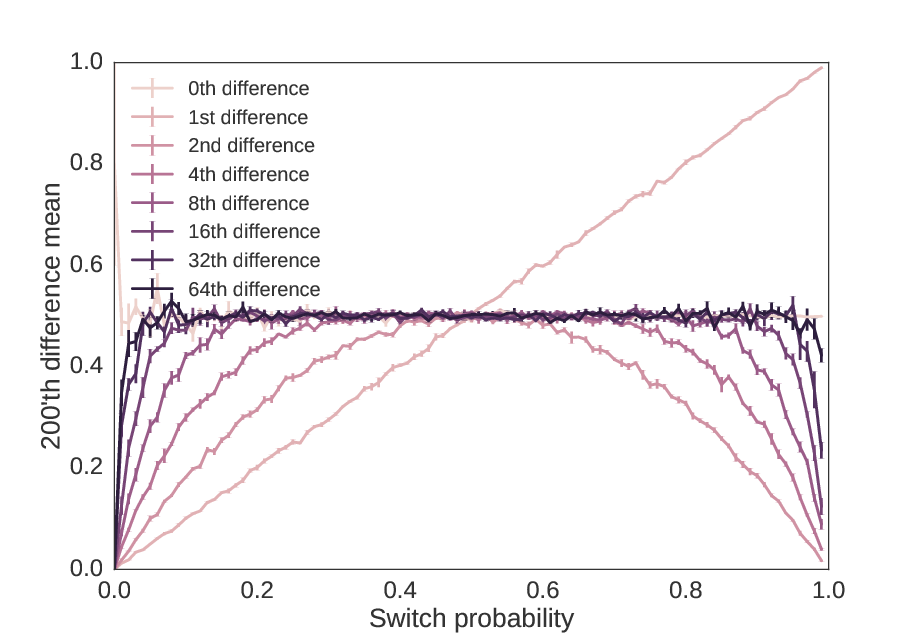
As we increase the precision by powers of two, we get sequences that have \(n\)‘th switch probabilities increasingly close to 50%, no matter what the 1st order switch probability was.
From this, it would be easy to conclude that the \(n\)‘th switch probability of a sequence approximates a random sequence as \(n → ∞\). But is this true? What if we do the powers of 2 plus one?
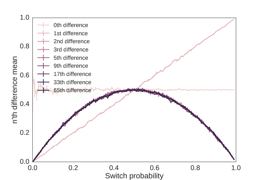
As we increase the precision by powers of two plus one, we get no closer to a random sequence than the 2nd order switch probability.
As we see, even though the switch probability approaches 50%, there is “hidden information” in the second order switch probability which makes this sequence non-random.
Is it possible?
Mathematicians have already figured out how we can turn biased coins (i.e. coins that have a \(p≠0.5\) probability of landing heads) into fair coin flips. This was famously described by Von Neumann. (While the Von Neumann procedure is not optimal, it is close, and its simplicity makes it appropriate for our purposes as a heuristic method.) To summarize this method, suppose you have a coin which comes up heads with a probability \(p≠0.5\). Then in order to obtain a random sequence, flip the coin twice. If the coins come up with the same value, discard both values. If they come up with different values, discard the second value. This takes on average \(n/(p-p^2)\) coin flips to generate a sequence of \(n\) values.
In our case, we want to correct for a biased switch probability. Thus, we must generate a sequence of random numbers, find the switches, apply this technique, and then map the switches back to the initial choices. So for example,
1011101000101011010100101000010
has switches at
110011100111110111110111100011
So converting this into pairs, we have
11 00 11 10 01 11 11 01 11 11 01 11 10 00 11
Applying the procedure, we get
1 0 0 0 1
and mapping it back, we get a random sequence of
100001
(With a bias of \(p=0.7\) in this example, the predicted length of our initial sequence of 31 was 6.5. This is a sequence of length 6.)
It is possible to recreate this precisely with a sliding window.
However, there is an easier way. In humans, the speed limiting step
is performing these calculations, not generating biased binary digits.
If we are willing to sacrifice theoretical efficiency (i.e. using as
few digits as possible) for simplicity, we can also look at our initial
sequence in chunks of 3. We then discard the sequences 101,
010, 111, and 000, but keep the most frequent digit
in the triple for the other observations, namely keeping a 0 for
001 and 100, or a 1 for 110, and 011.
(Note that this is only true because we assume an equal probability of
0 or 1 in the initial sequence. A more general choice
procedure would be a 0 if we observe 110 or 001, and
a 1 if we observe 100 or 011. However, this is more
difficult for humans to compute.) A proof that this method generates
truly random sequences is trivial.
When we apply this method to the sequences in Figures 1 and 2, we get the following, which shows both powers of two and powers of two plus one.
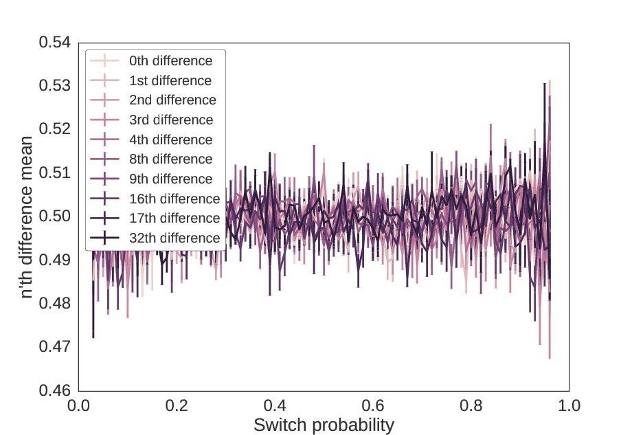
Using the triplet method, no differences of the sequence show
structure, i.e. the probability of a 0 or 1 is approximately 50%
in all differences. These values mimic those of the two previous
figures. The variance increases at the edges because the probability
of finding the triplets 010 and 101 is high when switch
probability is high, and the triplets 000 and 111 is high when
switch probability is low, so the resulting sequence is shorter.
Testing for randomness of these methods
While there are many definitions of random sequences, the normalized entropy is especially useful for our purposes. In short, normalized entropy divides the sequence into blocks of size \(k\) and looks at the probability of finding any given sequence of length \(k\). If it is a uniform probability, i.e. no block is any more likely than another block, the function gives a value of 1, but if some occur more frequently than others, it gives a value less than 1. In the extreme case where only one block appears, it gives a value of 0.
Intuitively, if we have a high switch probability, we would expect to
see the blocks 01 and 10 more frequently than 00 or 11.
Likewise, if we have a low switch probability, we would see more 00
and 11 blocks than 01 or 10. Similar relationships extend
beyond blocks of size 2. Entropy is useful for determining randomness
because it makes no assumptions about the form of the non-random
component.
As we can see below, the triplet method is identical to random, but all other methods show non-random patterns.
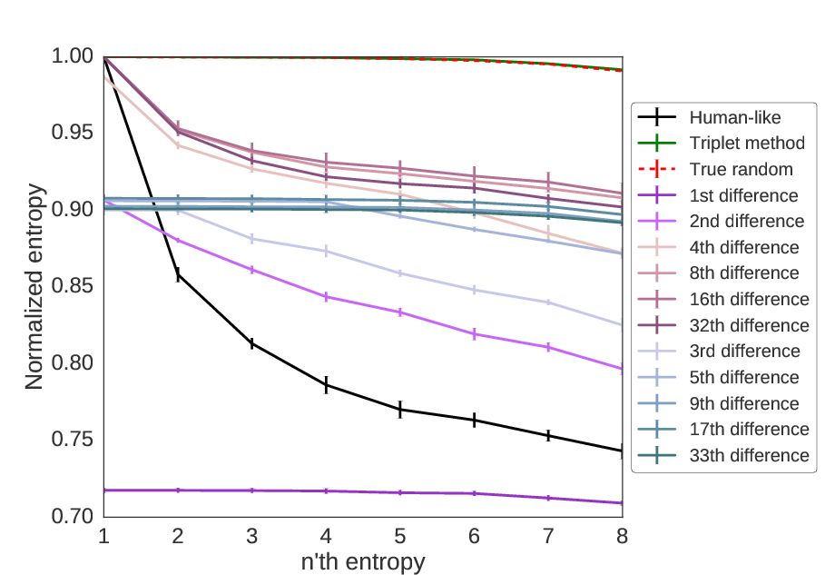
Using entropy, we can see which methods are able to mimic a random sequence. Of those we have considered here, only the triplet method is able to generate random values, as the normalized entropy is approximately equal to 1 for all sequence lengths.
Conclusions
Humans are not very effective at generating random numbers. With
random binary numbers, human-generated random numbers tend to switch
back and forth between sequences of 0s and 1s too quickly. Even
when made aware of this bias, it is difficult to compensate for it.
However, there may be ways that humans can generate sequences which
are closer to random sequences. One way is to split the sequence into
three-digit triplets, discarding the entire triplet for 000, 111,
010, and 101, and taking the most frequent number in all other
triplets. When the key non-random element is switch probability, this
creates an easy-to-compute method for generating a random binary
sequence.
Nevertheless, this triplet method relies on the assumption that the only bias humans have when generating random binary numbers is the switch probability bias. Since no data were analyzed here, it is still necessary to look into whether human-generated sequences have more non-random elements than just a change in switch probability.
More information
Technical notes
The 1st order switch sequence is also called differencing. Similarly, the sequence of \(n\)‘th order switches is equal to the \(n\)‘th difference. The 1st difference can also be thought of as a sliding XOR window, i.e. a parity sliding window of size 2.
Using the concept of a sliding XOR window raises the idea that the \(n\)‘th difference can be represented as as sliding parity window of size greater than 2. By construction, for a sequence of length \(N\), a sliding window of size \(k\) would end up producing a sequence of length \(N-k+1\). Since the \(n\)‘th difference produces a sequence of length \(N-n\), this means that a sliding window of length \(k\) would be limited to only the \((k-1)\)‘th difference.
It turns out that this can only be shown to hold for window sizes of powers of two. The proof by induction that this holds for window sizes of powers of two is a simple proof by induction. The 0th difference corresponds to a window of size 1. The parity of a single binary digit is just the digit itself. So it holds trivially in this case.
For the induction step, suppose the \((k-1)\)‘th difference is equal to the parity for a window of size \(k\) where \(k\) is a power of 2. Let \(x\) be any bit in at least the \((2k-1)\)‘th difference. Let the window of \(x\) be the appropriate window of \(2k\) digits of the original sequence which determines the value of \(x\). We need to show that the parity of the window of \(x\) is equal to the value of \(x\).
Without loss of generality, suppose the sequence of bits is of length \(2k\) (the window of \(x\)), and \(x\) is the single bit that is the \((2k-1)\)‘th difference.
Let us split the sequence in half, and apply the assumption to the first half and then to the second half separately. We notice that the parity of the parities of these halves is equal to the parity of the entire sequence. Splitting the sequence in half tells us that the first bit in the \((k-1)\)‘th difference is equal to the parity of the first half of the bits, and the second bit in the \((k-1)\)‘th difference is equal to the parity of the second half of the bits.
We can reason that these two bits would be equal iff the parity of the \(k\)‘th difference is 0, and different iff the parity of the \(k\)‘th difference is 1, because by the definition of a difference, we switch every time there is a 1 in the sequence, so an even number of switches means that the two bits would have the same parity. By applying our original assumption again, we know that if the \(k\)‘th difference is 0, then \(x\) will be 0, and if the \(k\)‘th difference is 1, \(x\) will be 1.
Therefore, \(x\) is equal to the parity of a window of size \(2k\), and hence the \((2k-1)\)‘th difference is equal to the parity of a sliding window of size \(2k\). QED.
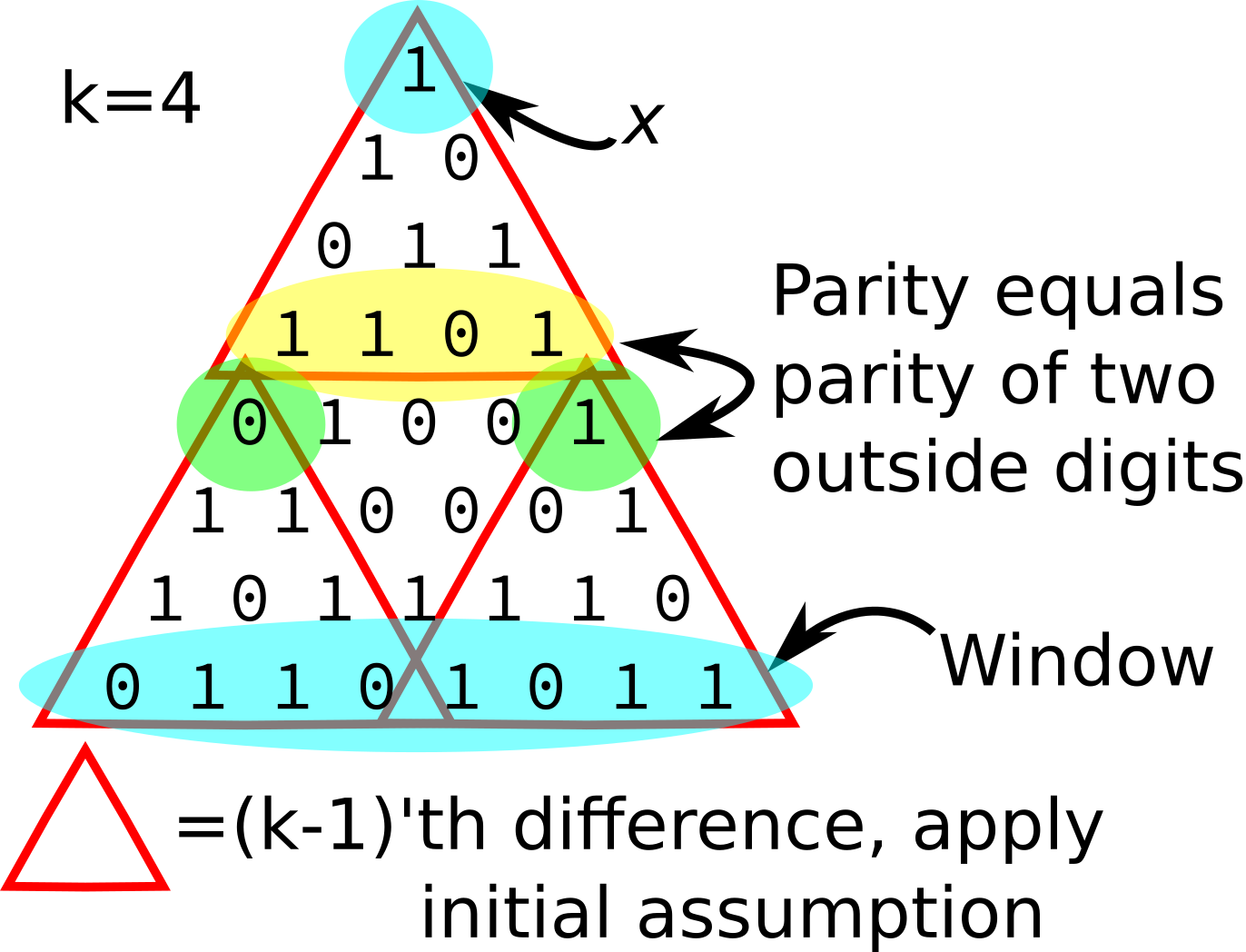
A visual version of the above proof.
Code/Data:
When to stop and when to keep going
I was recently posed the following puzzle:
Imagine you are offered a choice between two different bets. In (A), you must make 2/3 soccer shots, and in (B), you must make 5/8. In either case, you receive a \($100\) prize for winning the bet. Which bet should you choose?
Intuitively, a professional soccer player would want to take the second bet, whereas a hopeless case like me would want to take the first. However, suppose you have no idea whether your skill level is closer to Lionel Messi or to Max Shinn. The puzzle continues:
You are offered the option to take practice shots to determine your skill level at a cost of \($0.01\) for each shot. Assuming you and the goalie never fatigue, how do you decide when to stop taking practice shots and choose a bet?
Clearly it is never advisable to take more than \(100/.01=10000\) practice shots, but how many should we take? A key to this question is that you do not have to determine the number of shots to take beforehand. Therefore, rather than determining a fixed number of shots to take, we will instead need to determine a decision procedure for when to stop shooting and choose a bet.
There is no single “correct” answer to this puzzle, so I have documented my approach below.
Approach
To understand my approach, first realize that there are a finite number of potential states that the game can be in, and that you can fully define each state based on how many shots you have made and how many you have missed. The sum of these is the total number of shots you have taken, and the order does not matter. Additionally, we assume that all states exist, even if you will never arrive at that state by the decision procedure.
An example of a state is taking 31 shots, making 9 of them, and missing 22 of them. Another example is taking 98 shots, making 1 of them and missing 97 of them. Even though we may have already made a decision before taking 98 shots, the concept of a state does not depend on the procedure used to “get there”.
Using this framework, it is sufficient to show which decision we should take given what state we are in. My approach is as follows:
- Find a tight upper bound \(B \ll 10000\) on the number of practice shots to take. This limits the number of states to work with.
- Determine the optimal choice based on each potential state after taking \(B\) total shots. Once \(B\) shots have been taken, it is always best to have chosen either bet (A) or bet (B), so choose the best bet without the option of shooting again.
- Working backwards, starting with states with \(B-1\) shots and moving down to \(B-2,...,0\), determine the expected value of each of the three choices: select bet (A), select bet (B), or shoot again. Use this to determine the optimal choice to make at that position.
The advantage of this approach is that the primary criterion we will work with is the expected value for each decision. This means that if we play the game many times we will maximize the amount of money we earn. As a convenient consequence of this, we know much money we can expect to earn given our current state.
The only reason this procedure is necessary is because we don’t know our skill level. If we could determine with 100% accuracy what are skill level was, we would never need to take any shots at all. Thus, a key part of this procedure is estimating our skill level.
What if you know your skill level?
We define skill level as the probability \(p_0\) that you will make a shot. So if you knew your probability of making each shot, we could find your expected payoff from each bet. On the plot below, we show the payoff (in dollars) of each bet on the y-axis, and how it changes with skill on the x-axis.
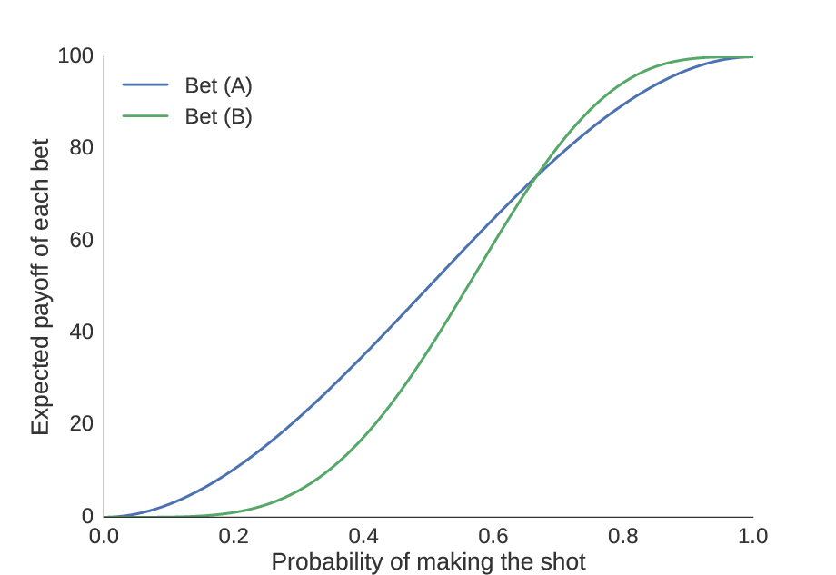
Assuming we have a precise knowledge of your skill level, we can find how much money you can expect to make from each bet.
The first thing to notice is the obvious: as our skill improves, the amount of money we can expect to win increases. Second, we see that there is some point (the “equivalence point”) at which the bets are equal; we compute this numerically to be \(p_0 = 0.6658\). We should choose bet (A) if our skill level is worse than \(0.6658\), and bet (B) if it is greater than \(0.6658\).
But suppose our guess is poor. We notice that the consequence for guessing too high is less than the consequence for guessing too low. It is better to bias your choice towards (A) unless you obtain substantial evidence that you have a high skill level and (B) would be a better choice. In other words, the potential gains from choosing (A) over (B) are larger than the potential gains for choosing (B) over (A).
Finding a tight upper bound
Quantifying this intuition, we compute the maximal possible gain of choosing (A) over (B) and (B) over (A) as the maximum distance between the curves on each side of the equivalence point. In other words, we find the skill level at which the incentive is strongest to choose one bet over the other, and then find what the incentive is at these points.
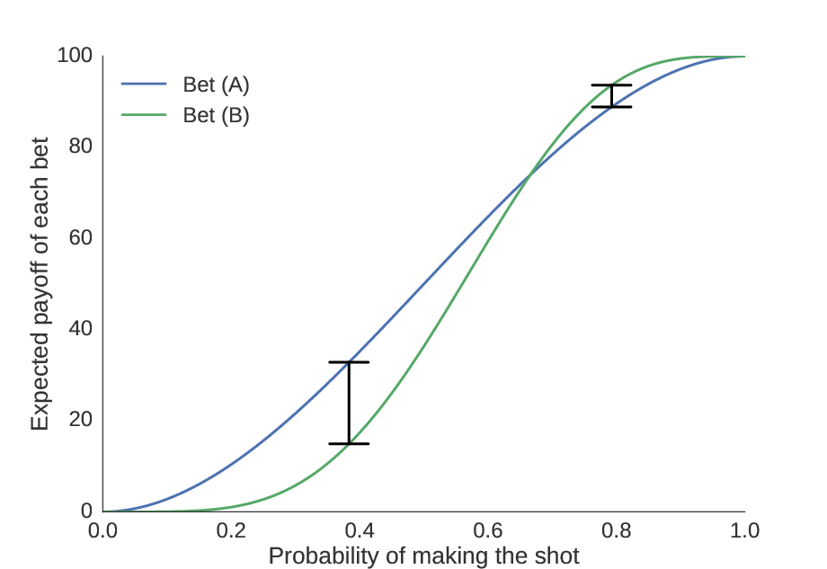
We see here the locations where the distance between the curves is greatest, showing the skill levels where it is most advantageous to choose (A) or (B).
This turns out to be \($4.79\) for choosing (B) over (A), and \($17.92\) for choosing (A) over (B). Since each shot costs \($0.01\), we conclude that it is never a good idea to take more than 479 practice shots. Thus, our upper bound \(B=479\).
Determining the optimal choice at the upper bound
Because we will never take more than 479 shots, we use this as a cutoff point, and force a decision once 479 shots have been taken. So for each possible combinations of successes and failures, we must find whether bet (A) or bet (B) is better.
In order to determine this, we need two pieces of information: first, we need the expected value of bets (A) and (B) given \(p_0\) (i.e. the curve shown above); second, we need the distribution representing our best estimate of \(p_0\). Remember, it is not enough to simply choose (A) when our predicted skill is less than \(0.6658\) and (B) when it is greater than \(0.6658\); since we are biased towards choosing (A), we need a probability distribution representing potential values of \(p_0\). Then, we can find the expected value of each bet given the distribution of \(p_0\) (see appendix for more details). This can be computed with a simple integral, and is easy to approximate numerically.
Once we have performed these computations, in addition to having information about whether (A) or (B) was chosen, we also know the expected value of the chosen bet. This will be critical for determining whether it is beneficial to take more shots before we have reached the upper bound.
Determining the optimal choice below the upper bound
We then go down one level: if 478 shots have been taken, with \(k\) successes and \((478-k)\) failures, should we choose (A), should we choose (B), or should we take another shot? Remember, we would like to select the choice which will give us the highest expected outcome.
Based on this principle, it is only advisable to take another shot if it would influence the outcome; in other words, if you would choose the same bet no matter what the outcome of your next shot, it does not make sense to take another shot, because you lose \($0.01\) without gaining any information. It only makes sense to take the shot if the information gained from taking the shot increases the expected value by more than \($0.01\).
Thus, we would only like to take another shot if the information gained is worth more than \($0.01\). We can compute this by finding the expected value of each of the three options (choose (A), choose (B), or shoot again). Using our previous experiments to judge the probability of a successful shot (see appendix), we can find the expected payoff of taking another shot. If it is greater than choosing (A) or (B), we take the shot.
Working backwards, we continue until we are on our first shot, where we assume we have a \(50\)% chance of succeeding. Once we reach this point, we have a full decision tree, indicating which action we should take based on the outcome of each shot, and the entire decision process can be considered solved.
Conclusion
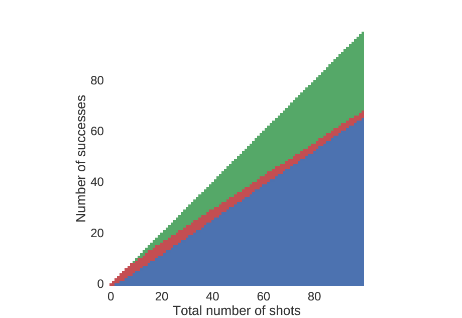
Here is the decision tree, plotted in raster form.
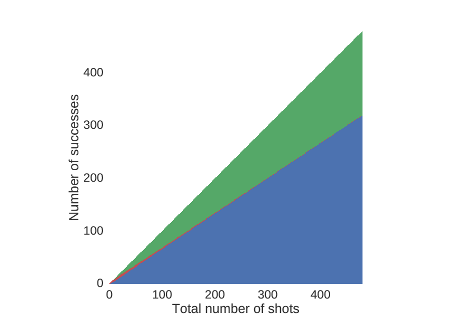
Starting at the point (0,0), go one to the right for every shot that you take, and one up for every shot that you make. Red indicates you should shoot again, blue indicates you should choose (A), and green indicates you should choose (B).
Looking more closely at the beginning, we see that unless you are really good, you should choose (A) rather quickly.
An identical plot to that above, but zoomed in near the beginning.
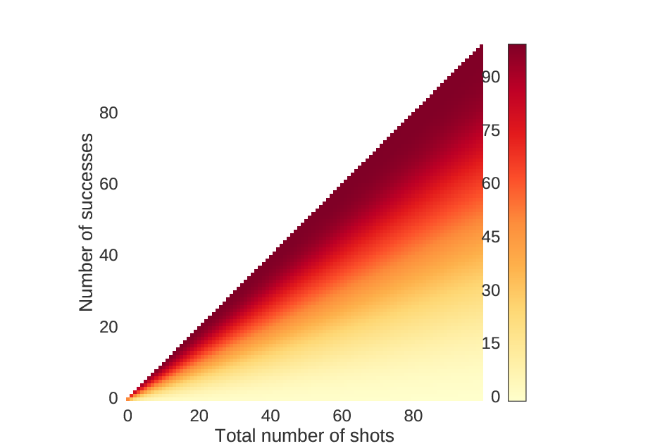
We can also look at the amount of money you will win on average if you play by this strategy. As expected, when you make more shots, you will have a higher chance of winning more money.

For each point in the previous figures, these values correspond to the choices.
We can also look at the zoomed in version.
An identical plot to the one above, but zoomed in near the beginning.
This algorithm grows in memory and computation time like \(O(B^2)\), meaning that if we double the size of the upper bound, we quadruple the amount of memory and CPU time we require.
This may not be the best strategy, but it seems to be a principled strategy which works reasonably well with a relatively small runtime.
Appendix: Determining the distribution of \(p_0\)
In order to find the distribution for \(p_0\), we consider the distribution of \(p_0\) for a single shot. The chance that we make a shot is \(100\)% if \(p_0=1\), \(0\)% if \(p_0=0\), \(50\)% if \(p_0=0.5\), and so on. Thus, the distribution of \(p_0\) from a single successful trial is \(f(p)=p\) for \(0 ≤ p ≤ 1\). Similarly, if we miss the shot, then the distribution is \(f(p)=(1-p)\) for \(0≤p≤1\). Since these probabilities are independent, we can multiply them together and find that, for \(n\) shots, \(k\) successes, and \((n-k)\) failures, we have \(f(p)=p^k (1-p)^{n-k}/c\) for some normalizing constant \(c\). It turns out, this is identical to the beta distribution, with parameters \(α=k+1\) and \(β=n-k+1\).
However, we need a point estimate of \(p_0\) to compute the expected value of taking another shot. We cannot simply use the ratio \(n/k\) for two practical reasons: first, it is undefined when no shots have been taken, and second, when the first shot has been taken, we have a \(100\)% probability of one outcome and a \(0\)% probability of the other. If we want to assume a \(50\)% probability of making the shot initially, an easy way to solve this problem is to use the ratio \((k+1)/(n+2)\) instead of \(k/n\) to estimate the probability. Interestingly, this quick and dirty solution is equivalent to finding the mean of the beta distribution. When no shots have been taken, \(k=0\) and \(n=0\), so \(α=1\) and \(β=1\), which is equivalent to the uniform distribution, hence our non-informative prior.
Code/Data:
Which hints are best in Towers?
There is a wonderful collection of puzzles by Simon Tatham called the Portable Puzzle Collection which serves as a fun distraction. The game “Towers” is a simple puzzle where you must fill in a Latin square with numbers \(1 \ldots N\), only one of each per row/column, as if the squares contained towers of this height. The number of towers visible from the edges of rows and columns are given as clues. For example,
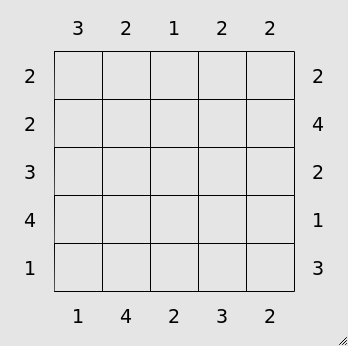
An example starting board from the Towers game.
Solved, the board would appear as,
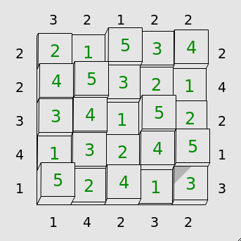
The previous example solved.
In more advanced levels, not all of the hints are given. Additionally, in these levels, hints can also be given in the form of the value of particular cells. For example, the initial conditions of the puzzle may be,
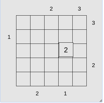
A more difficult example board.
With such different types of hints, it raises the question of whether some hints are better than others.
How will we approach the problem?
We will use an information-theoretic framework to understand how useful different hints are. This allows us to measure the amount of information that a particular hint gives about the solution to a puzzle in bits, a nearly-identical unit to that used by computers to measure file and memory size.
Information theory is based on the idea that random variables (quantities which can take on one of many values probabilistically) are not always independent, so sometimes knowledge of the value of one random variable can change the probabilities for a different random variable. For instance, one random variable may be a number 1-10, and a second random variable may be whether that number is even or odd. A bit is an amount of information equal to the best possible yes or no question, or (roughly speaking) information that can cut the number of possible outcomes in half. Knowing whether a number is even or odd gives us one bit of information, since it specifies that the first random variable can only be one of five numbers instead of one of ten.
Here, we will define a few random variables. Most importantly, we will have the random variable describing the correct solution of the board, which could be any possible board. We will also have random variables which represent hints. There are two types of hints: initial cell value hints (where one of the cells is already filled in) and tower visibility hints (which define how many towers are visible down a row or column).
The number of potential Latin squares of size \(N\) grows very fast. For a \(5×5\) square, there are 161,280 possibilities, and for a \(10×10\), there are over \(10^{47}\). Thus, for computational simplicity, we analyze a \(4×4\) puzzle with a mere 576 possibilities.
How useful are “initial cell value” hints?
First, we measure the entropy, or the maximal information content that
a single cell will give. For the first cell chosen, there is an equal
probability that any of the values (1, 2, 3, or 4) will be
found in that cell. Since there are two options, this give us 2 bits
of information.
What about the second initial cell value? Interestingly, it depends both on the location and on the value. If the second clue is in the same row or column as the first, it will give less information. If it is the same number as the first, it will also give less information.
Counter-intuitively, in the 4×4 board, this means we gain more than 2 bits of information from the second hint. This is because, once we reveal the first cell’s value, the probabilities of each of the other cell’s possible values are not equal as they were before. Since we are not choosing from the same row or column of our first choice, is more likely that this cell will be equal to the first cell’s value than to any other value. So therefore if we reveal a value which is different, it will provide more information.
Intuitively, for the 4×4 board, suppose we reveal the value of a cell
and it is 4. There cannot be another 4 in the same column or row,
so if we are to choose a hint from a different column or row, we are
effectively choosing from a leaving a 3×3 grid. There must be 3 4
values in the 3×3 grid, so the probability of selecting it is 1/3. We
have an even probability of selecting a 1, 2, or 3, so each
other symbol has a probability of 2/9. Being more surprising finds,
we gain 2.17 bits of information from each of these three.
Consequently, selecting a cell in the same row or column, or one which has the same value as the first, will give an additional 1.58 bits of information.
How about “tower visibility” hints?
In a 4×4 puzzle, it is very easy to compute the information gained if
the hint is a 1 or a 4. A hint of 1 always gives the same
amount of information as a single square: it tells us that the cell on
the edge of the hint must be a 4, and gives no information about the
rest of the squares. If only one tower can be seen, the tallest tower
must come first. Thus, it must give 2 bits of information.
Additionally, we know that if the hint is equal to 4, the only
possible combination for the row is 1, 2, 3, 4. Thus, this
gives an amount of information equal to the entropy of a single row,
which turns out to be 4.58 bits.
For a hint of 2 or 3, the information content is not as
immediately clear, but we can calculate them numerically. For a hint
of 2, we have 1.13 bits, and for a hint of 3, we have 2 bits.
Conveniently, due to the fact that the reduction of entropy in a row
must be equal to the reduction of entropy in the entire puzzle, we can
compute values for larger boards. Below, we show the information
gained about the solution from each possible hint (indicated by the
color). In general, it seems higher hints are usually better, but a
hint of 1 is generally better than one of 2 or 3.
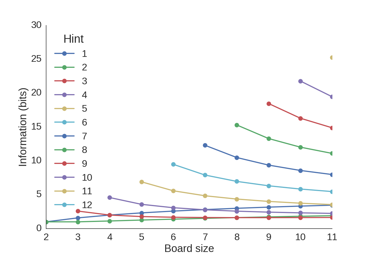
For each board size, the information content of each potential hint is plotted.
Conclusion
In summary:
- The more information given by a hint for a puzzle, the easier that hint makes it to solve the puzzle.
- Of the two types of hints, usually the hints about the tower visibility are best.
- On small boards (of size less than 5), hints about individual cells are very useful.
- The more towers visible from a row or column, the more information is gained about the puzzle from that hint.
Of course, remember that all of the hints combined of any given puzzle must be sufficient to completely solve the puzzle (assuming the puzzle is solvable), so the information content provided by the hints must be equal to the entropy of the puzzle of the given size. When combined, we saw in the “initial cell value” that hints may become more or less effective, so these entropy values cannot be directly added to determine which hints provide the most information. Nevertheless, this serves as a good starting point in determining which hints are the most useful.
More information
Theoretical note
For initial cell hints, it is possible to compute the information
content analytically for any size board. For a board of size \(N×N\)
with \(N\) symbols, we know that the information contained in the
first hint is \(-\log(1/N)\) bits. Suppose this play uncovers token
X. Using this first play, we construct a sub-board where the row
and column of the first hint are removed, leaving us with an
\((N-1)×(N-1)\) board. If we choose a cell from this board, it has a
\(1/(N-1)\) probability of being X and an equal chance of being
anything else, giving a \(\frac{N-2}{(N-1)^2}\) probability of each of
the other tokens. Thus, information gained is
\(-\frac{N-2}{(N-1)^2}×\log\left(\frac{N-2}{(N-1)^2}\right)\) if the
value is different from the first, and
\(-1/(N-1)×\log\left(1/(N-1)\right)\) if they are the same; these
expressions are approximately equal for large \(N\). Note how no
information is gained when the second square is revealed if \(N=2\).
Similarly, when a single row is revealed (for example by knowing that \(N\) towers are visible from the end of a row or column) we know that the entropy must be reduced by \(-\sum_{i=1}^N \log(1/N)\). This is because the first element revealed in the row gives \(-\log(1/N)\) bits, the second gives \(-\log(1/(N-1))\) bits, and so on.
Solving a puzzle algorithmically
Most of these puzzles are solvable without backtracking, i.e. the next move can always be logically deduced from the state of the board without the need for trial and error. By incorporating the information from each hint into the column and row states and then integrating this information across rows and columns, it turned out to be surprisingly simple to write a quick and dirty algorithm to solve the puzzles. This algorithm, while probably not of optimal computational complexity, worked reasonably well. Briefly,
- Represent the initial state of the board by a length-\(N\) list of lists, where each of the \(N\) lists represents a row of the board, and each sub-list contains all of the possible combinations of this row (there are \(N!\) of them to start). Similarly, define an equivalent (yet redundant) data structure for the columns.
- Enforce each condition on the start of the board by eliminating the impossible combinations using the number of towers visible from each row and column, and using the cells given at initialization. Update the row and column lists accordingly.
- Now, the possible moves for certain squares will be restricted by the row and column limitations; for instance, if only 1 tower is visible in a row or column, the tallest tower in the row or column must be on the edge of the board. Iterate through the cells, restricting the potential rows by the limitations on the column and vice versa. For example, if we know the position of the tallest tower in a particular column, eliminate the corresponding rows which do not have the tallest tower in this position in the row.
- After sufficient iterations of (3), there should only be one possible ordering for each row (assuming it is solvable without backtracking). The puzzle is now solved.
This is not a very efficient algorithm, but it is fast enough and memory-efficient enough for all puzzles which might be fun for a human to solve. This algorithm also does not work with puzzles which require backtracking, but could be easily modified to do so.
Code/Data:
When should you leave for the bus?
Anyone who has taken the bus has at one time or another wondered, “When should I plan to be at the bus stop?” or more importantly, “When should I leave if I want to catch the bus?” Many bus companies suggest arriving a few minutes early, but there seem to be no good analyses on when to leave for the bus. I decided to find out.
Finding a cost function
Suppose we have a bus route where a bus runs every \(I\) minutes, so if you don’t catch your bus, you can always wait for the next bus. However, since more than just your time is at stake for missing the bus (e.g. missed meetings, stress, etc.), we assume there is a penalty \(\delta\) for missing the bus in addition to the extra wait time. \(\delta\) here is measured in minutes, i.e. how many minutes of your time would you exchange to be guaranteed to avoid missing the bus. \(\delta=0\) therefore means that you have no reason to prefer one bus over another, and that you only care about minimizing your lifetime bus wait time.
Assuming we will not be late enough to need to catch the third bus, we can model this with two terms, representing the cost to you (in minutes) of catching each of the next two buses, weighted by the probability that you will catch that bus:
\[C(t) = \left(E(T_B) - t\right) P\left(T_B > t + L_W\right) + \left(I + E(T_B) - t + \delta\right) P(T_B < t + L_W)\]where \(T_B\) is the random variable representing the time at which the bus arrives, \(L_W\) is the random variable respresenting the amount of time it takes to walk to the bus stop, and \(t\) is the time you leave. (\(E\) is expected value and \(P\) is the probability.) We wish to choose a time to leave the office \(t\) which minimizes the cost function \(C\).
If we assume that \(T_B\) and \(L_W\) are Gaussian, then it can shown that the optimal time to leave (which minimizes the above function) is
\[t = -\mu_W - \sqrt{\left(\sigma_B^2 + \sigma_W^2\right)\left(2\ln\left(\frac{I+\delta}{\sqrt{\sigma_B^2+\sigma_W^2}}\right)-2\ln\left(\sqrt{2\pi}\right)\right)}\]where \(\sigma_B^2\) is the variance of the bus arrival time, \(\sigma_W^2\) is the variance of your walk, and \(\mu_W\) is expected duration of your walk. In other words, you should plan to arrive at the bus stop on average \(\sqrt{\left(\sigma_B^2 + \sigma_W^2\right)\left(2\ln\left(\left(I+\delta\right)/\sqrt{\sigma_B^2+\sigma_W^2}\right)-2\ln\left(\sqrt{2\pi}\right)\right)}\) minutes before your bus arrives.
Note that one deliberate oddity of the model is that the cost function does not just measure wait time, but also walking time. I optimized on this because, in the end, what matters is the total time you spend getting on the bus.
What does this mean?
The most important factor you should consider when choosing which bus to take is the variability in the bus’ arrival time and the variability in the time it takes you to walk to the bus. The arrival time scales approximately linearly with the standard deviation of the variability.
Additionally, it scales at approximately the square root of the log the your value of time and of the frequency of the buses. So even if very high values of time and very infrequent buses do not substantially change the time at which you should arrive. For approximation purposes, you might consider adding a constant in place of this term, anywhere from 2-5 minutes depending on the frequency of the bus.
Checking the assumption
First, we need to collect some data to assess whether the bus time arrival (\(T_B\)) is normally distributed. I wrote scripts to scrape data from Yale University’s Blue Line campus shuttle route. Many bus systems (including Yale’s) now have real-time predictions, so I used many individual predictions by Yale’s real-time arrival prediction system as the expected arrival time, simulating somebody checking this to see when the next bus comes.
For our purposes, the expected arrival time looks close enough to a Gaussian distribution:
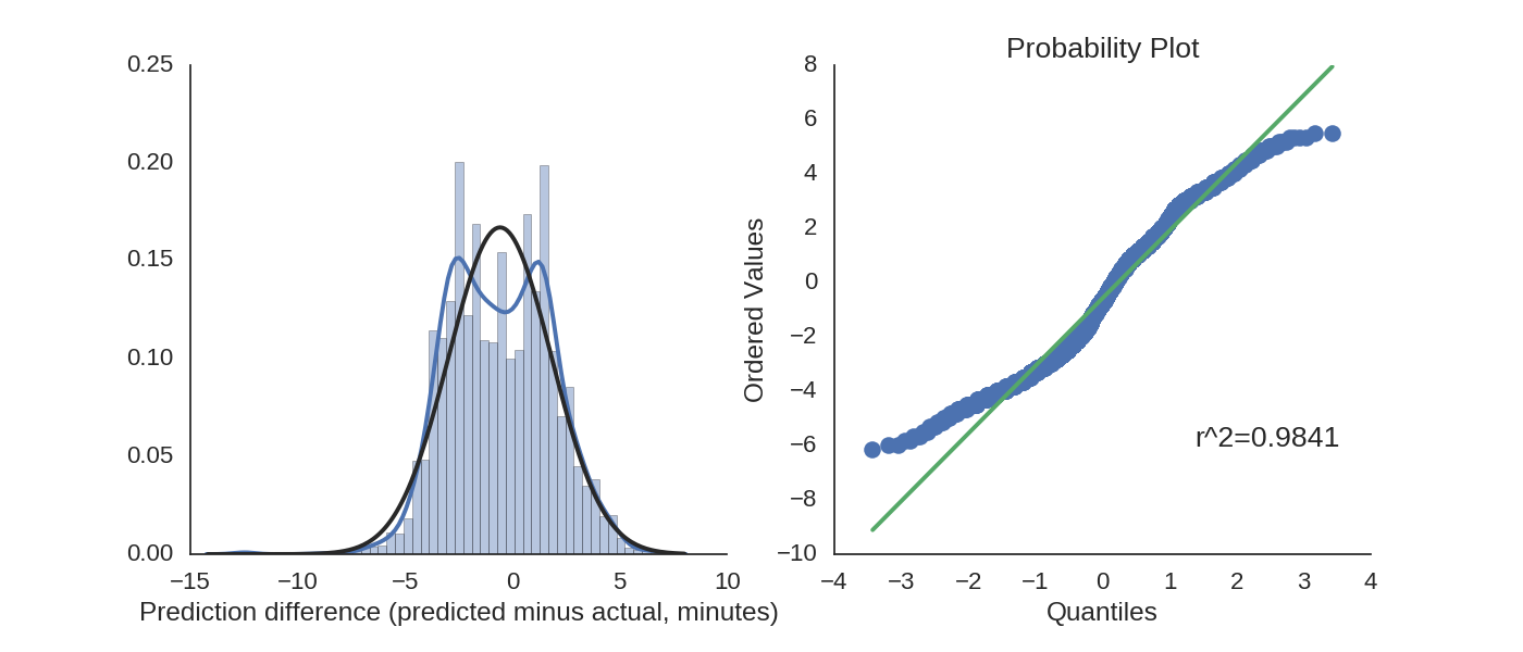
It actually looks like a Gaussian!
So what time should I leave?
When estimating the \(\sigma_B^2\) parameter, we only examine bus times which are 10 minutes away or later. This is because you can’t use a real-time bus system to plan ahead of time to catch something if it is too near in the future, which defeats the purpose of the present analysis. The variance in arrival time for the Yale buses is \(\sigma_B^2=5.7\).
We use an inter-bus interval of \(I=15\) minutes.
While the variability of the walk to the bus station \(\sigma_W^2\) is unique for each person, I consider two cases: one case, where we assume that arrival time variability is small (\(\sigma_W^2=0\)) compared to the bus’ variability, representing the case where the bus stop is (for intance) located right outside one’s office building. I also consider the case where the time variability is comperable to the variability for the bus (\(\sigma_W=5\)), representing the case where one must walk a long distance to the bus stop.
Finally, I consider the case where we strongly prioritize catching the desired bus (\(\delta=60\) corresponding to, e.g., an important meeting) and also the case where we seek to directly minimize the expected wait time (\(\delta=0\) corresponding to, e.g., the commute home).
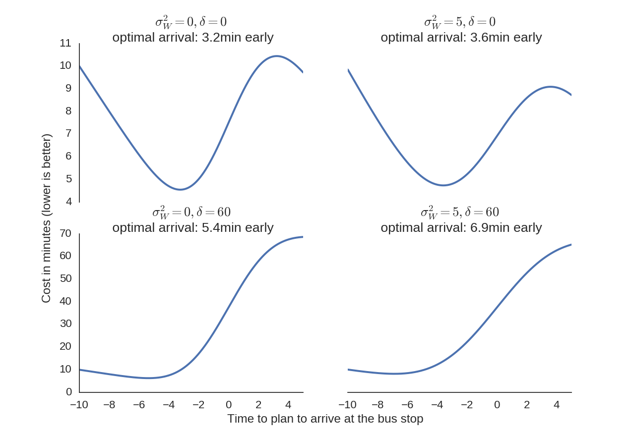
Even though the shape of the optimization function changes greatly, the optimal arrival time changes very little.
We can also look at a spectrum of different cost tradeoffs for missing the bus (values of \(\delta\)) and variance in the walk time (values of \(\sigma_W^2 = var(W)\)). Because they appear similarly in the equations, we can also consider these values to be changes in the interval of the bus arrival \(I\) and the variance of the bus’ arrival time \(\sigma_B^2=var(B)\) respectively.
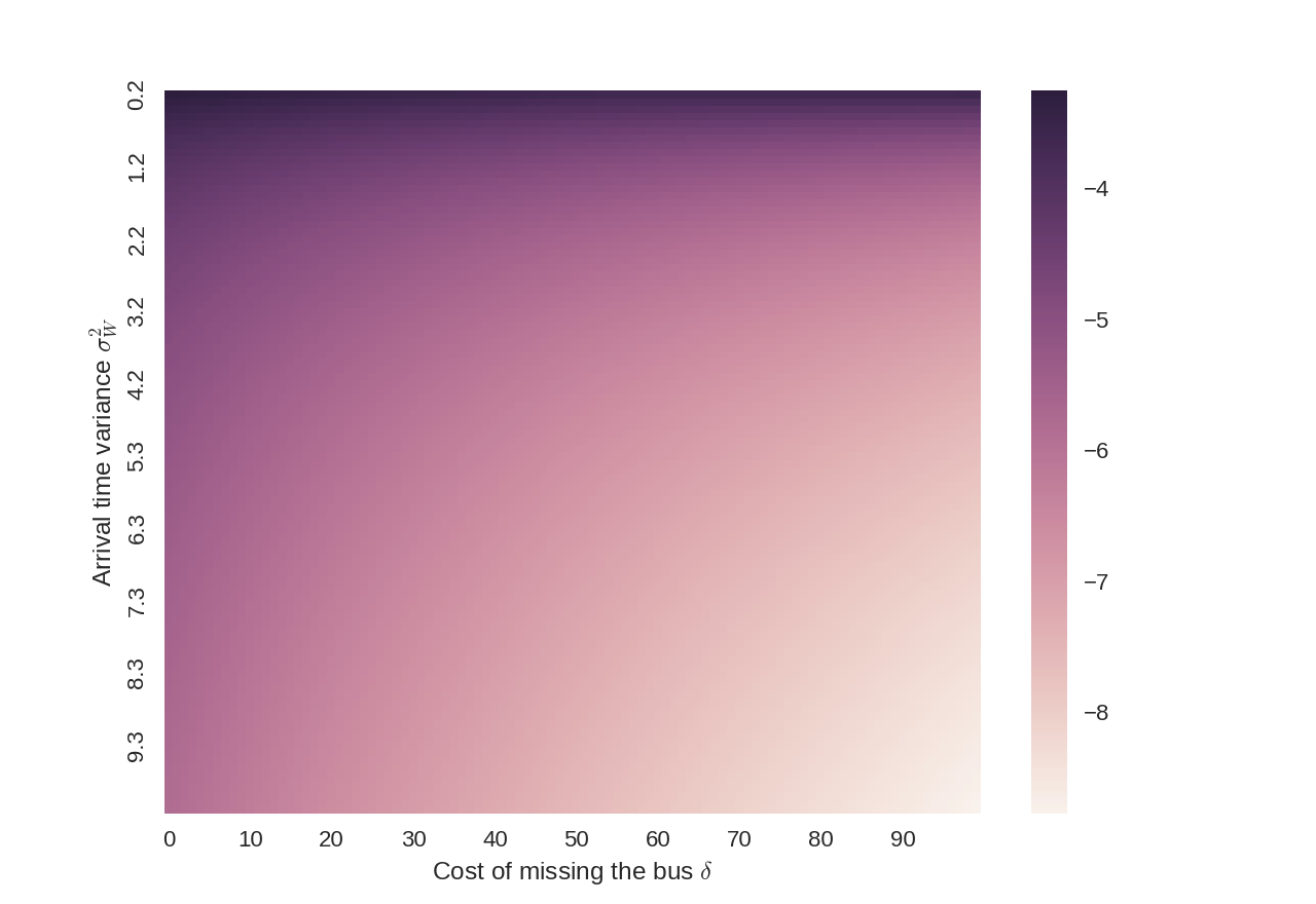
Across all reasonable values, the optimal time to plan to arrive is between 3.5 and 8 minutes early.
Conclusion
So to summarize:
- If it always takes you approximately the same amount of time to walk to the bus stop, plan to be there 3-4 minutes early on your commute home, or 5-6 minutes early if it’s the last bus before an important meeting.
- If you have a long walk to the bus stop which can vary in duration, plan to arrive at the bus stop 4-5 minutes early if you take the bus every day, or around 7-8 minutes early if you need to be somewhere for a special event.
- These estimations assume that you know how long it takes you on average to walk to the bus stop. As we saw previously, if you need to be somewhere at a certain time, arriving a minute early is much better than arriving a minute late. If you don’t need to be somewhere, just make your best guess.
- The best way to reduce waiting time is to decrease variability.
- These estimates also assume that the interval between buses is sufficiently large. If it is small, as in the case of a subway, there are different factors that govern the time you spend waiting.
- This analysis focuses on buses with an expected arrival time, not with a scheduled arrival time. When buses have schedules, they will usually wait at the stop if they arrive early. This situation would require a different analysis than what was performed here.